Visium HD: colonrectal cancer
Last updated: 2025-04-14
Checks: 6 1
Knit directory: KODAMA-Analysis/
This reproducible R Markdown analysis was created with workflowr (version 1.7.1). The Checks tab describes the reproducibility checks that were applied when the results were created. The Past versions tab lists the development history.
The R Markdown file has unstaged changes. To know which version of
the R Markdown file created these results, you’ll want to first commit
it to the Git repo. If you’re still working on the analysis, you can
ignore this warning. When you’re finished, you can run
wflow_publish to commit the R Markdown file and build the
HTML.
Great job! The global environment was empty. Objects defined in the global environment can affect the analysis in your R Markdown file in unknown ways. For reproduciblity it’s best to always run the code in an empty environment.
The command set.seed(20240618) was run prior to running
the code in the R Markdown file. Setting a seed ensures that any results
that rely on randomness, e.g. subsampling or permutations, are
reproducible.
Great job! Recording the operating system, R version, and package versions is critical for reproducibility.
Nice! There were no cached chunks for this analysis, so you can be confident that you successfully produced the results during this run.
Great job! Using relative paths to the files within your workflowr project makes it easier to run your code on other machines.
Great! You are using Git for version control. Tracking code development and connecting the code version to the results is critical for reproducibility.
The results in this page were generated with repository version 5f5ac63. See the Past versions tab to see a history of the changes made to the R Markdown and HTML files.
Note that you need to be careful to ensure that all relevant files for
the analysis have been committed to Git prior to generating the results
(you can use wflow_publish or
wflow_git_commit). workflowr only checks the R Markdown
file, but you know if there are other scripts or data files that it
depends on. Below is the status of the Git repository when the results
were generated:
Ignored files:
    Ignored:    .RData
    Ignored:    .Rhistory
    Ignored:    .Rproj.user/

Untracked files:
    Untracked:  KODAMA.svg
    Untracked:  analysis/singlecell_datamatrix.Rmd
    Untracked:  analysis/singlecell_seurat.Rmd
    Untracked:  code/Acinar_Cell_Carcinoma.ipynb
    Untracked:  code/Adenocarcinoma.ipynb
    Untracked:  code/Adjacent_normal_section.ipynb
    Untracked:  code/DLFPC_preprocessing.R
    Untracked:  code/DLPFC - BANKSY.R
    Untracked:  code/DLPFC - BASS.R
    Untracked:  code/DLPFC - BAYESPACE.R
    Untracked:  code/DLPFC - Nonspatial.R
    Untracked:  code/DLPFC - PRECAST.R
    Untracked:  code/DLPFC_comparison.R
    Untracked:  code/DLPFC_results_analysis.R
    Untracked:  code/MERFISH - BANKSY.R
    Untracked:  code/MERFISH - BASS.R
    Untracked:  code/MERFISH - BAYESPACE.R
    Untracked:  code/MERFISH - Nonspatial.R
    Untracked:  code/MERFISH - PRECAST.R
    Untracked:  code/MERFISH_comparison.R
    Untracked:  code/MERFISH_results_analysis.R
    Untracked:  code/VisiumHD-CRC.ipynb
    Untracked:  code/VisiumHDassignment.py
    Untracked:  code/deep learning code DLPFC.R
    Untracked:  code/save tiles.py
    Untracked:  data/Annotations/
    Untracked:  data/DLFPC-Br5292-input.RData
    Untracked:  data/DLFPC-Br5595-input.RData
    Untracked:  data/DLFPC-Br8100-input.RData
    Untracked:  data/DLPFC-general.RData
    Untracked:  data/MERFISH-input.RData
    Untracked:  data/trajectories.RData
    Untracked:  data/trajectories_VISIUMHD.RData
    Untracked:  output/BANSKY-results.RData
    Untracked:  output/BASS-results.RData
    Untracked:  output/BayesSpace-results.RData
    Untracked:  output/CRC-image.RData
    Untracked:  output/CRC-image2.RData
    Untracked:  output/CRC.png
    Untracked:  output/CRC2.png
    Untracked:  output/CRC7.png
    Untracked:  output/CRC8.png
    Untracked:  output/CRC_boxplot.png
    Untracked:  output/CRC_boxplot.svg
    Untracked:  output/CRC_boxplot2.svg
    Untracked:  output/CRC_linee.svg
    Untracked:  output/DL.RData
    Untracked:  output/DLFPC-All-2.RData
    Untracked:  output/DLFPC-All.RData
    Untracked:  output/DLFPC-Br5292.RData
    Untracked:  output/DLFPC-Br5595.RData
    Untracked:  output/DLFPC-Br8100.RData
    Untracked:  output/DLFPC-variablesXdeeplearning.RData
    Untracked:  output/DLPFC-BANSKY-results.RData
    Untracked:  output/DLPFC-BASS-results.RData
    Untracked:  output/DLPFC-BayesSpace-results.RData
    Untracked:  output/DLPFC-Nonspatial-results.RData
    Untracked:  output/DLPFC-PRECAST-results.RData
    Untracked:  output/DLPFC_all_cluster.svg
    Untracked:  output/DLPFCpathway.RData
    Untracked:  output/Figure 1 - boxplot.pdf
    Untracked:  output/Figure 2 - DLPFC 10.pdf
    Untracked:  output/Figures/
    Untracked:  output/KODAMA-results.RData
    Untracked:  output/KODAMA_DLPFC_All_original.svg
    Untracked:  output/KODAMA_DLPFC_Br5595.svg
    Untracked:  output/KODAMA_DLPFC_Br5595_slide.svg
    Untracked:  output/Loupe.csv
    Untracked:  output/MERFISH-BANSKY-results.RData
    Untracked:  output/MERFISH-BASS-results.RData
    Untracked:  output/MERFISH-BayesSpace-results.RData
    Untracked:  output/MERFISH-KODAMA-results.RData
    Untracked:  output/MERFISH-Nonspatial-results.RData
    Untracked:  output/MERFISH-PRECAST-results.RData
    Untracked:  output/MERFISH.RData
    Untracked:  output/Nonspatial-results.RData
    Untracked:  output/Prostate-GSEA.csv
    Untracked:  output/Prostate-KODAMA.RData
    Untracked:  output/Prostate-trajectory.csv
    Untracked:  output/Prostate.RData
    Untracked:  output/VisiumHD-RNA.RData
    Untracked:  output/VisiumHD-genes.pdf
    Untracked:  output/VisiumHD.RData
    Untracked:  output/boh.svg
    Untracked:  output/desmoplastic_distance_carcinoma.csv
    Untracked:  output/image.RData
    Untracked:  output/pp.RData
    Untracked:  output/pp2.RData
    Untracked:  output/pp3.RData
    Untracked:  output/pp4.RData
    Untracked:  output/pp5.RData
    Untracked:  output/prostate1.svg
    Untracked:  output/prostate2.svg
    Untracked:  output/prostate3.svg
    Untracked:  output/subclusters1.csv
    Untracked:  output/subclusters2.csv
    Untracked:  output/subclusters3.csv
    Untracked:  output/tight_boundary.geojson
    Untracked:  output/trajectory.csv

Unstaged changes:
    Deleted:    analysis/D1.Rmd
    Deleted:    analysis/DLPFC-12.Rmd
    Deleted:    analysis/DLPFC-4.Rmd
    Modified:   analysis/DLPFC.Rmd
    Deleted:    analysis/DLPFC1.Rmd
    Deleted:    analysis/DLPFC10.Rmd
    Deleted:    analysis/DLPFC2.Rmd
    Deleted:    analysis/DLPFC3.Rmd
    Deleted:    analysis/DLPFC4.Rmd
    Deleted:    analysis/DLPFC5.Rmd
    Deleted:    analysis/DLPFC6.Rmd
    Deleted:    analysis/DLPFC7.Rmd
    Deleted:    analysis/DLPFC8.Rmd
    Deleted:    analysis/DLPFC9.Rmd
    Deleted:    analysis/Du1.Rmd
    Deleted:    analysis/Du10.Rmd
    Deleted:    analysis/Du11.Rmd
    Deleted:    analysis/Du12.Rmd
    Deleted:    analysis/Du13.Rmd
    Deleted:    analysis/Du14.Rmd
    Deleted:    analysis/Du15.Rmd
    Deleted:    analysis/Du16.Rmd
    Deleted:    analysis/Du17.Rmd
    Deleted:    analysis/Du18.Rmd
    Deleted:    analysis/Du19.Rmd
    Deleted:    analysis/Du2.Rmd
    Deleted:    analysis/Du20.Rmd
    Deleted:    analysis/Du3.Rmd
    Deleted:    analysis/Du4.Rmd
    Deleted:    analysis/Du5.Rmd
    Deleted:    analysis/Du6.Rmd
    Deleted:    analysis/Du7.Rmd
    Deleted:    analysis/Du8.Rmd
    Deleted:    analysis/Du9.Rmd
    Modified:   analysis/Giotto.Rmd
    Modified:   analysis/MERFISH.Rmd
    Deleted:    analysis/MERFISH1a (copy).Rmd
    Deleted:    analysis/MERFISH1a.Rmd
    Deleted:    analysis/MERFISH1b (copy).Rmd
    Deleted:    analysis/MERFISH1b.Rmd
    Deleted:    analysis/MERFISH2a (copy).Rmd
    Deleted:    analysis/MERFISH2a.Rmd
    Deleted:    analysis/MERFISH2b (copy).Rmd
    Deleted:    analysis/MERFISH2b.Rmd
    Deleted:    analysis/MERFISH3a (copy).Rmd
    Deleted:    analysis/MERFISH3a.Rmd
    Deleted:    analysis/MERFISH3b (copy).Rmd
    Deleted:    analysis/MERFISH3b.Rmd
    Deleted:    analysis/MERFISH4a (copy).Rmd
    Deleted:    analysis/MERFISH4a.Rmd
    Deleted:    analysis/MERFISH4b (copy).Rmd
    Deleted:    analysis/MERFISH4b.Rmd
    Modified:   analysis/Prostate.Rmd
    Deleted:    analysis/STARmap.Rmd
    Modified:   analysis/Seurat.Rmd
    Deleted:    analysis/Simulation.Rmd
    Deleted:    analysis/Single-cell.Rmd
    Modified:   analysis/SpatialExperiment.Rmd
    Modified:   analysis/VisiumHD.Rmd
    Modified:   code/VisiumHD_CRC_download.sh
    Deleted:    data/Pathology.csv
    Deleted:    data/merfish.Rmd
    Deleted:    data/vis.R
Note that any generated files, e.g. HTML, png, CSS, etc., are not included in this status report because it is ok for generated content to have uncommitted changes.
These are the previous versions of the repository in which changes were
made to the R Markdown (analysis/VisiumHD.Rmd) and HTML
(docs/VisiumHD.html) files. If you’ve configured a remote
Git repository (see ?wflow_git_remote), click on the
hyperlinks in the table below to view the files as they were in that
past version.
| File | Version | Author | Date | Message |
|---|---|---|---|---|
| html | 5b7dd63 | Stefano Cacciatore | 2025-01-10 | Build site. |
| Rmd | 86be707 | Stefano Cacciatore | 2025-01-10 | Start my new project |
| Rmd | 7bba919 | Stefano Cacciatore | 2025-01-09 | Start my new project |
| html | a423e5f | Stefano Cacciatore | 2024-09-04 | Build site. |
| Rmd | b0a97fe | Stefano Cacciatore | 2024-09-04 | Start my new project |
| html | 9bdaa70 | Stefano Cacciatore | 2024-09-04 | Build site. |
| Rmd | ca72951 | Stefano Cacciatore | 2024-09-04 | Start my new project |
| html | 098b08e | Stefano Cacciatore | 2024-09-04 | Build site. |
| Rmd | eb8066e | Stefano Cacciatore | 2024-09-04 | Start my new project |
| html | 0010f3c | Stefano Cacciatore | 2024-09-04 | Build site. |
| Rmd | 3f515c0 | Stefano Cacciatore | 2024-09-04 | Start my new project |
| html | 51b0452 | Stefano Cacciatore | 2024-09-03 | Build site. |
| Rmd | c257b0e | Stefano Cacciatore | 2024-09-03 | Start my new project |
| Rmd | 22e2ac6 | Stefano Cacciatore | 2024-08-26 | Start my new project |
| html | d1192e9 | Stefano Cacciatore | 2024-08-12 | Build site. |
| Rmd | 5ef8148 | Stefano Cacciatore | 2024-08-12 | Start my new project |
| html | 3374e66 | Stefano Cacciatore | 2024-08-06 | Build site. |
| html | 35ce733 | Stefano Cacciatore | 2024-08-03 | Build site. |
| html | 82fe167 | Stefano Cacciatore | 2024-07-24 | Build site. |
| Rmd | b422e43 | Stefano Cacciatore | 2024-07-24 | Start my new project |
| html | 6f7daac | Stefano Cacciatore | 2024-07-19 | Build site. |
| Rmd | 5b97082 | tkcaccia | 2024-07-15 | updates |
| Rmd | 7be8f59 | tkcaccia | 2024-07-15 | updates |
| html | 7be8f59 | tkcaccia | 2024-07-15 | updates |
| Rmd | 79f73a2 | GitHub | 2024-07-14 | Update VisiumHD.Rmd |
| html | f8ca54a | tkcaccia | 2024-07-14 | update |
| html | d04c1e7 | GitHub | 2024-07-08 | Update VisiumHD.html |
| html | 754c8bf | GitHub | 2024-07-04 | Update VisiumHD.html |
| html | ee4ee17 | GitHub | 2024-06-19 | Add files via upload |
| Rmd | 615fc05 | GitHub | 2024-06-19 | Add files via upload |
Introduction
The recently released VisiumHD platform by 10x Genomics significantly improves spatial transcriptomics resolution by reducing the spot size from 55 µm to an edge length of just 2 µm. This advancement eliminates gaps between spots, enabling truly gap-free and bias-free single-cell resolution. The high-density array allows for flexible data analysis at multiple resolutions, enabling researchers to tailor spatial granularity to specific biological questions. In the following analysis, we applied KODAMA to data at an 8 µm resolution.
Loading and Preprocessing Data
The dataset can be downloaded using the following script: VisiumHD_CRC_download.sh. This script provides access to the raw data, which will be preprocessed and analyzed in the subsequent steps of our pipeline.
The dataset will be then loaded in the R environment using the Seurat pipeline.
library("ggplot2")
library("patchwork")
library("dplyr")
library("Seurat")
library("KODAMA")
library("KODAMAextra")
library("bigmemory")

localdir="../Colorectal/outs/"
object <- Load10X_Spatial(data.dir = localdir, bin.size = c(8))
We perform quality control on a spatial transcriptomics dataset by removing low-quality spots with fewer than 100 UMIs, filtering out mitochondrial genes, and retaining genes expressed with at least 1 count in at least 0.5% of spots. The remaining high-quality genes are set as variable features for downstream analysis.
nCount_Spatial=colSums(object@assays$Spatial.008um$counts)


sp_obj <- subset(
  object,
  subset = nCount_Spatial.008um > 100)

nCount_Spatial=colSums(sp_obj@assays$Spatial.008um$counts)


counts=sp_obj@assays$Spatial.008um$counts
is_mito <- grepl("(^MT-)|(^mt-)", rownames(counts))
counts <- counts[!is_mito,]

filter_genes_ncounts=1
filter_genes_pcspots=0.5
nspots <- ceiling(filter_genes_pcspots/100 *  ncol(counts))
ix_remove <- rowSums(counts >= filter_genes_ncounts) <   nspots
counts <- counts[!ix_remove,]

QCgenes <- rownames(counts)

VariableFeatures(sp_obj) = QCgenes

rm(counts)
We prepare the filtered spatial transcriptomics data for dimensionality reduction using principal component analysis (PCA). We set the default assay, normalize the data, identify variable features, and scale the data. We then extract the tissue coordinates and we perform PCA using the filtered genes, storing the result as “pca.008um”. Finally, PCA is displayed in a scatterplot.
DefaultAssay(sp_obj) <- "Spatial.008um"
sp_obj <- NormalizeData(sp_obj)


sp_obj <- FindVariableFeatures(sp_obj)
sp_obj <- ScaleData(sp_obj)

xy=as.matrix(GetTissueCoordinates(sp_obj)[,1:2])

sp_obj <- RunPCA(sp_obj, reduction.name = "pca.008um")

dim(sp_obj)
[1] 18085 428381plot(Seurat::Embeddings(sp_obj, reduction = "pca.008um"))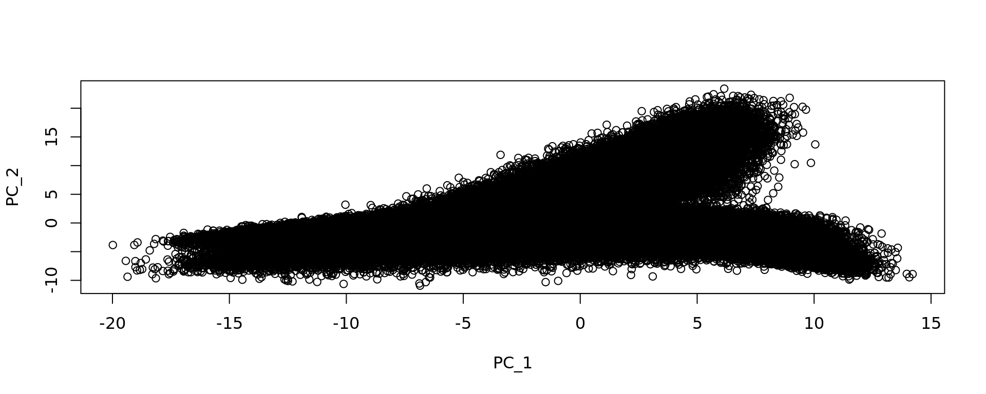
KODAMA analysis
We performed the KODAMA analysis using as input the 50 principal components of PCA and using 10000 landmarks.
n.cores=8

sp_obj=RunKODAMAmatrix(sp_obj,
                       reduction = "pca.008um",
                       landmarks = 10000,
                       n.cores=n.cores,
                       seed = 543210)

config <- umap.defaults
config$n_threads = n.cores
config$n_sgd_threads = "auto"

sp_obj=RunKODAMAvisualization(sp_obj,method="UMAP",config=config)


kk_UMAP=Seurat::Embeddings(sp_obj, reduction = "KODAMA")
Tissue annotation
The tissue was manually annotated using QuPath software and the annotations were save in Visium_HD_Human_Colon_Cancer_290325.geojson.
Using the script VisiumHDassignment.py the annotations saved as *.geojson were assigned to the Visium spots and saved in spots_classification_VisiumHD.csv.
rr=read.csv("data/Annotations/spots_classification_VisiumHD.csv",sep=",")
ss=strsplit(rr[,2],":")
ss=unlist(lapply(ss, function(x) x[2]))
ss=strsplit(ss,",")
ss=unlist(lapply(ss, function(x) x[1]))
ss=gsub("\"","",ss)

rr[,2]=ss
n=ave(1:length(rr[,1]), rr[,1], FUN = seq_along)
rr=rr[n==1,]
rownames(rr)=rr[,1]
rr=rr[rownames(kk_UMAP),]

rr[,2]=substring(rr[,2],2)

table(rr[,"classification"])
            blood vessel   desmoplastic submucosa                dysplasia
                    1969                    55409                    89290
dystrophic calcification            exocrine duct          external glands
                     488                      158                     3108
            immune cells   intramucosal carcinoma      intratumoral stroma
                    2713                    69214                    13336
      invasive carcinoma lamina propria dysplasia  lymphovascular channels
                   37283                    26834                     1505
       muscularis mucosa       muscularis propria             nerve fibers
                    4785                    18023                      457
            normal gland    normal lamina propria     oedematous submucosa
                   30199                    16502                     5865
library(ggplot2)
cols=sample(rainbow(15))
labels=as.factor(rr[,"classification"])
cols_tissue <- c("#0000ff", "#e41a1c", "#006400", "#00cc8f" ,"#0088dd",
"#00ff00", "#b2dfee","#669bbc", "#81b29a", "#ffd700",
"#adc178", "#aa1133", "#1166dc", "#e5989b", "#e07a5f",
"#cc00b6", "#81ccff", "#f2cc8f","#e0aa5f","#33b233", "#aa228f","#aa7a6f")
df <- data.frame(kk_UMAP[,1:2], tissue=labels)
plot1 = ggplot(df, aes(Dimensions_1, Dimensions_2, color = tissue)) +labs(title="KODAMA") +
geom_point(size = 1) +
theme_bw() + theme(legend.position = "bottom")+
scale_color_manual("Domain", values = cols_tissue) +
guides(color = guide_legend(nrow = 4,
override.aes = list(size = 4)))
plot1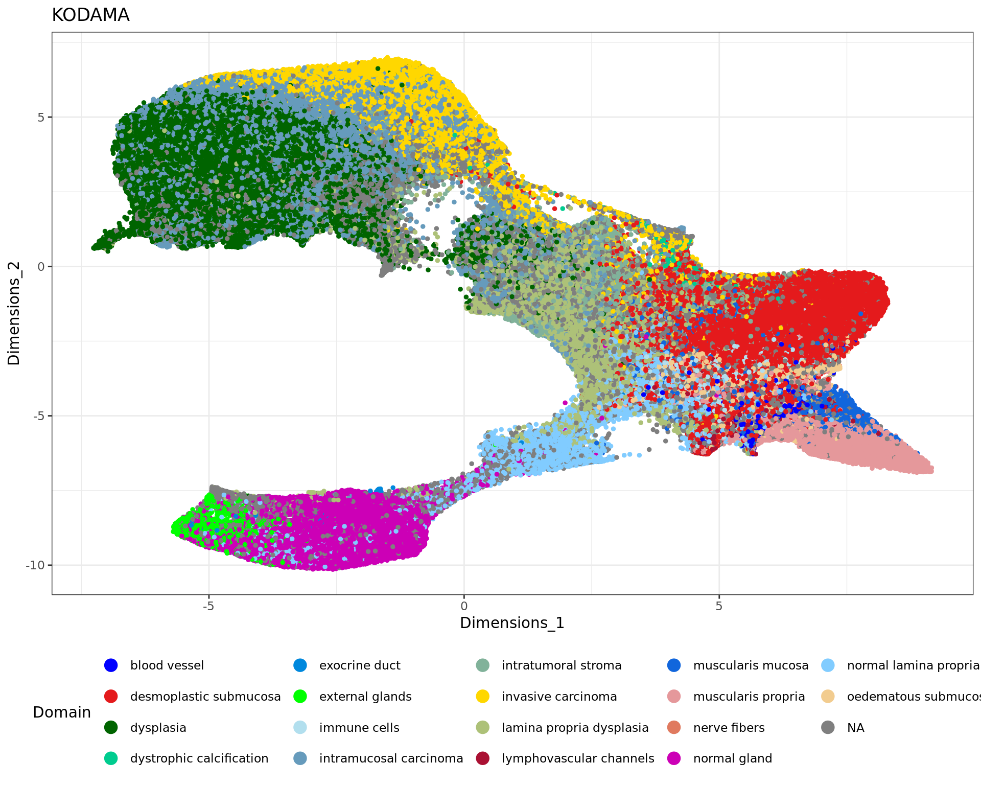
Trajectory analysis
The function new_trajectory allows us to draw manually a trajectory into the KODAMA plot to identify the gradual changes in the gene expression. The trajectory were previously drew and saved in the file trajectories_VISIUMHD.RData.
par(xpd = T, mar = par()$mar + c(0,0,0,7))


data=sp_obj@assays$Spatial.008um$data[rownames(sp_obj@assays$Spatial.008um$scale.data),]
data=as.matrix(data)
Warning in asMethod(object): sparse->dense coercion: allocating vector of size
6.4 GiBdata=t(data)
data=data[,-which(colMeans(data==0)>0.99)]load("data/trajectories_VISIUMHD.RData")
plot(kk_UMAP,cex=0.5,pch=20,col=cols_tissue[labels])
legend(max(kk_UMAP[,1])+0.05*dist(range(kk_UMAP[,1])), max(kk_UMAP[,2]),
levels(labels),
col = cols,
cex = 0.8,
pch=20)
mm1=new_trajectory (kk_UMAP,data = data,trace=tra1$xy)
mm2=new_trajectory (kk_UMAP,data = data,trace=tra2$xy)
mm3=new_trajectory (kk_UMAP,data = data,trace=tra3$xy)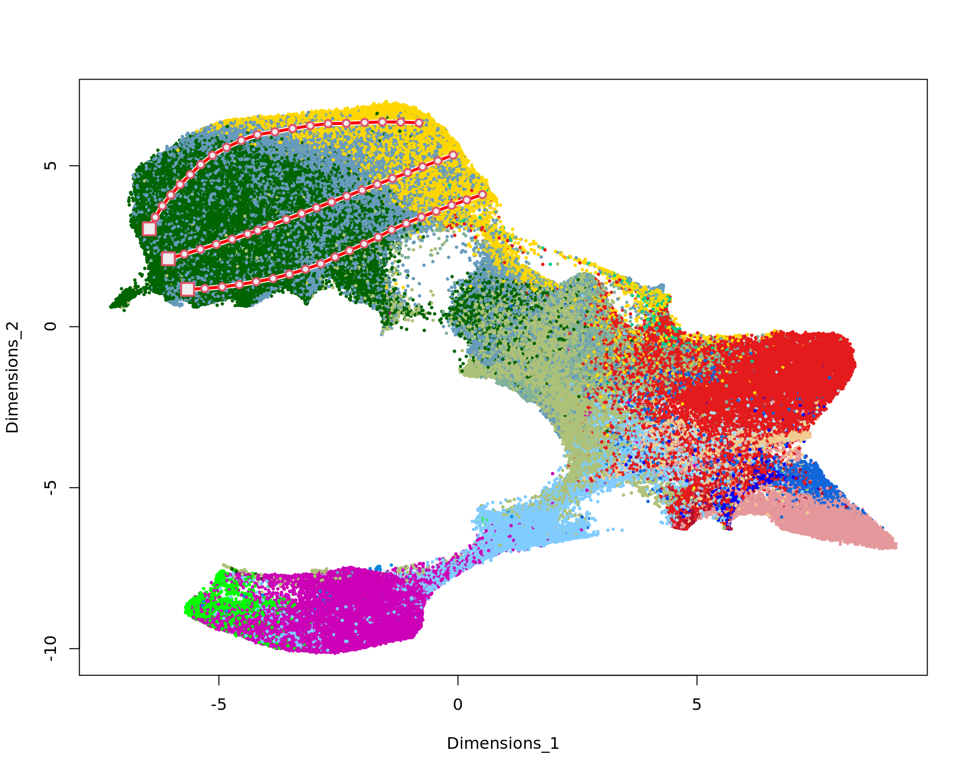
traj=rbind(mm1$trajectory,
           mm2$trajectory,
           mm3$trajectory)
y=rep(1:20,3)
The genes were were correlated with the trajectory using the Spearman correlation test.
ma=multi_analysis(traj,y,FUN="correlation.test",method="spearman")
ma=ma[order(as.numeric(ma$`p-value`)),]
colnames(ma)=c("Feature   ","rho   ","p-value   ","FDR   ")
knitr::kable(ma[1:10,],row.names=FALSE)| Feature | rho | p-value | FDR |
|---|---|---|---|
| LCN2 | -0.88 | 6.92e-21 | 6.94e-18 |
| SOD2 | -0.81 | 3.83e-15 | 1.92e-12 |
| CEBPD | -0.81 | 5.75e-15 | 1.92e-12 |
| CXCL3 | -0.77 | 7.34e-13 | 1.67e-10 |
| ID1 | -0.77 | 8.35e-13 | 1.67e-10 |
| IL32 | -0.75 | 4.17e-12 | 6.97e-10 |
| PI3 | -0.74 | 1.34e-11 | 1.91e-09 |
| CCL20 | -0.74 | 1.73e-11 | 2.17e-09 |
| CXCL1 | -0.74 | 2.16e-11 | 2.40e-09 |
| TRIM31 | -0.73 | 2.89e-11 | 2.90e-09 |
Validation of the results in the COAD TCGA cohort
The downregulation of CXCL3 across the progression of the carcinoma was validated using the RNAseq data of the COAD TGCA cohort. Clinical and gene expression data were downloaded from FireBrowse.
# install.packages("readxl")
library(readxl)

# Read in Clinical Data:
coad=read.csv("../TCGA/COAD/COAD.clin.merged.picked.txt",sep="\t",check.names = FALSE, row.names = 1)
coad <- as.data.frame(coad)

# Clean column names: replace dots with dashes & convert to uppercase
colnames(coad) = toupper(colnames(coad))

 # Transpose the dataframe so that rows become columns and vice versa
coad = t(coad)
Prepare RNA-seq expression data:
# Read RNA-seq expression data:
r = read.csv("../TCGA/COAD/COAD.rnaseqv2__illuminahiseq_rnaseqv2__unc_edu__Level_3__RSEM_genes_normalized__data.data.txt", sep = "\t", check.names = FALSE, row.names = 1)
# Remove the first row:
r = r[-1,]
# Convert expression data to numeric matrix format
temp = matrix(as.numeric(as.matrix(r)), ncol=ncol(r))
colnames(temp) = colnames(r)
rownames(temp) = rownames(r)
RNA = temp

# Transpose the matrix so that genes are rows and samples are columns
RNA = t(RNA)
Extract patient and tissue information from column names:
tcgaID = list()
 # Extract sample ID
tcgaID$sample.ID <- substr(colnames(r), 1, 16)
# Extract patient ID
tcgaID$patient <- substr(colnames(r), 1, 12)
# Extract tissue type
tcgaID$tissue <- substr(colnames(r), 14, 16)

tcgaID = as.data.frame(tcgaID)
Select Primary Solid Tumor tissue data (“01A”):
sel=tcgaID$tissue == "01A"
tcgaID.sel = tcgaID[sel, ]

# Subset the RNA expression data to match selected samples
RNA.sel = RNA[sel, ]
Intersect patient IDs between clinical and RNA data:
sel = intersect(tcgaID.sel$patient, rownames(coad))
# Subset the clinical data to include only selected patients:
coad.sel = coad[sel, ]
# Assign patient IDs as row names to the RNA data:
rownames(RNA.sel) = tcgaID.sel$patient
# Subset the RNA data to include only selected patients
RNA.sel = RNA.sel[sel, ]
Prepare labels for pathology stages:
The tumor samples were classified based on their T stage: -
t1, t2, & t3 as “low” -
t4, t4a, & t4b as “high” -
tis stages to NA
labelsTCGA = coad.sel[, "pathology_T_stage"]
labelsTCGA[labelsTCGA %in% c("t1", "t2", "t3", "tis")] = "low"
labelsTCGA[labelsTCGA %in% c("t4", "t4a", "t4b")] = "high"
table(labelsTCGA)
labelsTCGA
high low
38 242 Boxplot to visualize the distribution of log transformed gene expression by pathology stage:
colors=c("#0073c2bb","#efc000bb","#868686bb","#cd534cbb","#7aabdcbb","#003c67bb")

library(ggpubr)

gene.selected="CXCL3"
gene.selected.RNA=colnames(RNA.sel)[pmatch(gene.selected,colnames(RNA.sel))]

CXCL3 <- log(1 + RNA.sel[, gene.selected.RNA])
df=data.frame(variable=CXCL3,labels=labelsTCGA)

my_comparisons=list()
my_comparisons[[1]]=c(1,2)

Nplot1=ggboxplot(df, x = "labels", y = "variable",fill="labels",
                 width = 0.8,
                 palette=colors,
                 add = "jitter",
                 add.params = list(size = 2, jitter = 0.2,fill="#ff0000aa", shape=21))+
  ylab("CXCL3 gene expression (FPKM)")+ xlab("")+
  stat_compare_means(comparisons = my_comparisons,method="wilcox.test")

Nplot1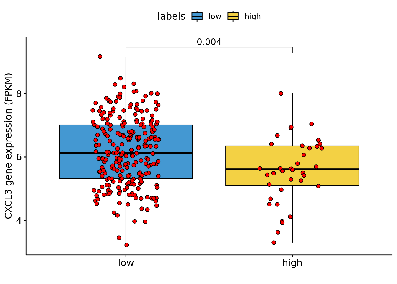
xy2=xy
xy2[,1]=xy[,2]
xy2[,2]=-xy[,1]

df <- data.frame(xy2, tissue=labels)
plot2 = ggplot(df, aes(x, y, color = tissue)) +labs(title="KODAMA") +
  geom_point(size = 1) +
  theme_bw() + theme(legend.position = "bottom")+
  scale_color_manual("Domain", values = cols_tissue) +
  guides(color = guide_legend(nrow = 4,
                              override.aes = list(size = 4)))
plot2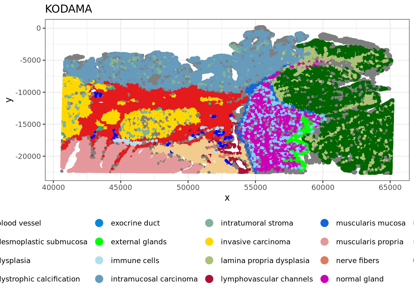
Proximity analysis
The gene expression of the desmoplastic submucosa are analyzed. The genes with gene expression correlates with the distance from the invasive carcinoma are identified.
sel_desmoplastic_submucosa=which(labels=="desmoplastic submucosa")
xy_desmoplastic_submucosa=xy[sel_desmoplastic_submucosa,]
data_desmoplastic_submucosa=data[sel_desmoplastic_submucosa,]
data_desmoplastic_submucosa=data_desmoplastic_submucosa[,-which(colMeans(data_desmoplastic_submucosa==0)>0.95)]
dim(data_desmoplastic_submucosa)
[1] 55409 201sel_invasive_carcinoma=which(labels=="invasive carcinoma" | labels=="intramucosal carcinoma")
xy_invasive_carcinoma=xy[sel_invasive_carcinoma,]
knn=Rnanoflann::nn(xy_invasive_carcinoma,xy_desmoplastic_submucosa,1)
y=knn$distances[,1]# Define custom intervals
break_points <-c(quantile(y,probs=c(seq(0,1,0.005))))
# Convert continuous data to intervals
distance_binned <- cut(y, breaks = break_points)
gene_binned=apply(data_desmoplastic_submucosa,2,function(x) tapply(x,distance_binned,mean))
break_points=break_points[-length(break_points)]
ma=multi_analysis(gene_binned,break_points,FUN="correlation.test",method="MINE")
ma=ma[order(as.numeric(ma$MIC),decreasing = TRUE),]
rownames(ma)=ma[,"Feature"]
knitr::kable(ma[1:20,],row.names=FALSE)| Feature | MIC | p-value | FDR |
|---|---|---|---|
| IGFBP5 | 1.00 | 3.9e-239 | 3.92e-237 |
| HTRA3 | 1.00 | 9.1e-261 | 1.83e-258 |
| MGP | 0.99 | 7.32e-191 | 3.68e-189 |
| TIMP3 | 0.92 | 1.88e-171 | 6.31e-170 |
| GREM1 | 0.91 | 4.3e-206 | 2.88e-204 |
| IGFBP3 | 0.89 | 4.32e-176 | 1.74e-174 |
| SFRP4 | 0.86 | 1.84e-170 | 5.29e-169 |
| CXCL14 | 0.84 | 9.84e-148 | 1.80e-146 |
| COL1A1 | 0.83 | 7.49e-152 | 1.67e-150 |
| MMP11 | 0.80 | 1.07e-141 | 1.66e-140 |
| SPARC | 0.76 | 1.99e-128 | 2.50e-127 |
| AEBP1 | 0.76 | 6.24e-99 | 5.23e-98 |
| CCDC80 | 0.75 | 2.47e-129 | 3.31e-128 |
| SFRP2 | 0.75 | 3.47e-90 | 2.49e-89 |
| ISLR | 0.75 | 3.13e-161 | 7.88e-160 |
| COL1A2 | 0.74 | 7.6e-102 | 7.27e-101 |
| DCN | 0.74 | 5.3e-98 | 4.26e-97 |
| COL3A1 | 0.73 | 6.96e-132 | 9.99e-131 |
| COL14A1 | 0.73 | 2.01e-100 | 1.83e-99 |
| A2M | 0.73 | 2.73e-99 | 2.38e-98 |
 df=data.frame(x=break_points,
               HTRA3=gene_binned[,"HTRA3"],
               IGFBP5=gene_binned[,"IGFBP5"],
               CXCL14=gene_binned[,"CXCL14"],
               MMP11=gene_binned[,"MMP11"],
               TIMP3=gene_binned[,"TIMP3"],
               MGP=gene_binned[,"MGP"],
               GREM1=gene_binned[,"GREM1"],
               IGFBP3=gene_binned[,"IGFBP3"],
               SFRP4=gene_binned[,"SFRP4"])

 ll=loess(IGFBP5~x,data = df,span = 0.3)
 IGFBP5=predict(ll,newdata = data.frame(x=break_points))

 ll=loess(CXCL14~x,data = df,span = 0.3)
 CXCL14=predict(ll,newdata = data.frame(x=break_points))

 ll=loess(MMP11~x,data = df,span = 0.3)
 MMP11=predict(ll,newdata = data.frame(x=break_points))

 ll=loess(TIMP3~x,data = df,span = 0.3)
 TIMP3=predict(ll,newdata = data.frame(x=break_points))

 ll=loess(HTRA3~x,data = df,span = 0.3)
 HTRA3=predict(ll,newdata = data.frame(x=break_points))

 ll=loess(MGP~x,data = df,span = 0.3)
 MGP=predict(ll,newdata = data.frame(x=break_points))


 ll=loess(GREM1~x,data = df,span = 0.3)
 GREM1=predict(ll,newdata = data.frame(x=break_points))


 ll=loess(IGFBP3~x,data = df,span = 0.3)
 IGFBP3=predict(ll,newdata = data.frame(x=break_points))


 ll=loess(SFRP4~x,data = df,span = 0.3)
 SFRP4=predict(ll,newdata = data.frame(x=break_points))


cols_lines <- c( "#006400", "#00cc8f" ,"#0088dd",
                  "#b2dfee", "#ffd700",   "#adc178", "#aa1133", "#e07a5f",
                 "#cc00b6", "#f2cc8f", "#aa228f","#aa7a6f")

plot(log(1+break_points),gene_binned[,1],ylim=c(0,1),type="n")


 points(log(1+break_points),HTRA3/max(HTRA3),type="l",col=cols_lines[1],lwd=3)
 points(log(1+break_points),IGFBP5/max(IGFBP5),type="l",col=cols_lines[2],lwd=3)
 points(log(1+break_points),CXCL14/max(CXCL14),type="l",col=cols_lines[3],lwd=3)
 points(log(1+break_points),MMP11/max(MMP11),type="l",col=cols_lines[4],lwd=3)
 points(log(1+break_points),TIMP3/max(TIMP3),type="l",col=cols_lines[5],lwd=3)
 points(log(1+break_points),MGP/max(MGP),type="l",col=cols_lines[6],lwd=3)
 points(log(1+break_points),GREM1/max(GREM1),type="l",col=cols_lines[7],lwd=3)
 points(log(1+break_points),IGFBP3/max(IGFBP3),type="l",col=cols_lines[8],lwd=3)
 points(log(1+break_points),SFRP4/max(SFRP4),type="l",col=cols_lines[9],lwd=3)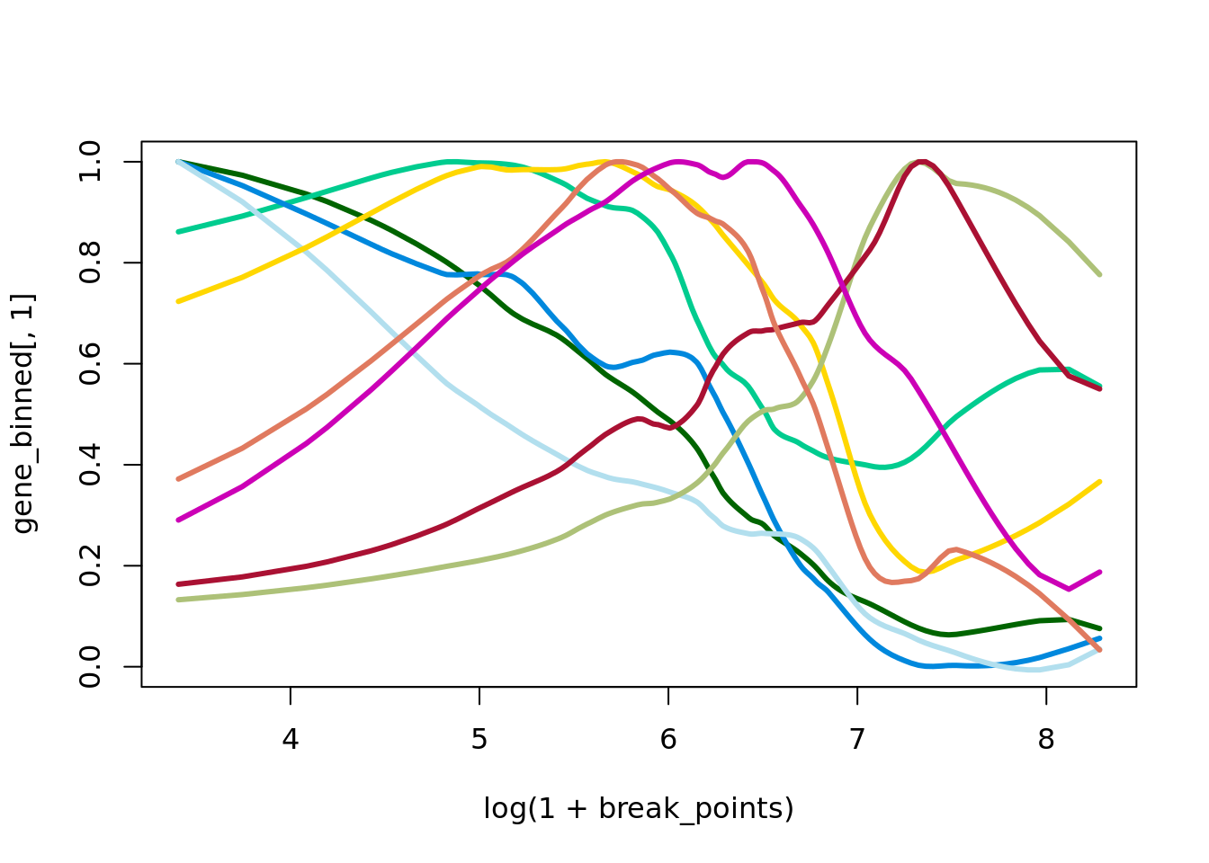
sessionInfo()R version 4.4.3 (2025-02-28)
Platform: x86_64-pc-linux-gnu
Running under: Ubuntu 20.04.6 LTS
Matrix products: default
BLAS: /usr/lib/x86_64-linux-gnu/blas/libblas.so.3.9.0
LAPACK: /usr/lib/x86_64-linux-gnu/lapack/liblapack.so.3.9.0
locale:
[1] LC_CTYPE=en_US.UTF-8 LC_NUMERIC=C
[3] LC_TIME=en_US.UTF-8 LC_COLLATE=en_US.UTF-8
[5] LC_MONETARY=en_US.UTF-8 LC_MESSAGES=en_US.UTF-8
[7] LC_PAPER=en_US.UTF-8 LC_NAME=C
[9] LC_ADDRESS=C LC_TELEPHONE=C
[11] LC_MEASUREMENT=en_US.UTF-8 LC_IDENTIFICATION=C
time zone: Etc/UTC
tzcode source: system (glibc)
attached base packages:
[1] parallel stats graphics grDevices utils datasets methods
[8] base
other attached packages:
[1] ggpubr_0.6.0 readxl_1.4.5 bigmemory_4.6.4 KODAMAextra_1.2
[5] e1071_1.7-16 doParallel_1.0.17 iterators_1.0.14 foreach_1.5.2
[9] KODAMA_3.0 Matrix_1.7-3 umap_0.2.10.0 Rtsne_0.17
[13] minerva_1.5.10 Seurat_5.2.1 SeuratObject_5.0.2 sp_2.2-0
[17] dplyr_1.1.4 patchwork_1.3.0 ggplot2_3.5.1 workflowr_1.7.1
loaded via a namespace (and not attached):
[1] RcppAnnoy_0.0.22 splines_4.4.3 later_1.4.1
[4] tibble_3.2.1 cellranger_1.1.0 polyclip_1.10-7
[7] fastDummies_1.7.5 lifecycle_1.0.4 tcltk_4.4.3
[10] rstatix_0.7.2 rprojroot_2.0.4 globals_0.16.3
[13] processx_3.8.6 Rnanoflann_0.0.3 lattice_0.22-7
[16] hdf5r_1.3.12 MASS_7.3-65 backports_1.5.0
[19] magrittr_2.0.3 plotly_4.10.4 sass_0.4.9
[22] rmarkdown_2.29 jquerylib_0.1.4 yaml_2.3.10
[25] httpuv_1.6.15 sctransform_0.4.1 spam_2.11-1
[28] askpass_1.2.1 spatstat.sparse_3.1-0 reticulate_1.42.0
[31] cowplot_1.1.3 pbapply_1.7-2 RColorBrewer_1.1-3
[34] abind_1.4-8 purrr_1.0.4 misc3d_0.9-1
[37] git2r_0.33.0 ggrepel_0.9.6 irlba_2.3.5.1
[40] listenv_0.9.1 spatstat.utils_3.1-3 goftest_1.2-3
[43] RSpectra_0.16-2 spatstat.random_3.3-3 fitdistrplus_1.2-2
[46] parallelly_1.43.0 codetools_0.2-20 tidyselect_1.2.1
[49] farver_2.1.2 matrixStats_1.5.0 spatstat.explore_3.4-2
[52] jsonlite_2.0.0 Formula_1.2-5 progressr_0.15.1
[55] ggridges_0.5.6 survival_3.8-3 tools_4.4.3
[58] ica_1.0-3 Rcpp_1.0.14 glue_1.8.0
[61] gridExtra_2.3 xfun_0.51 withr_3.0.2
[64] fastmap_1.2.0 openssl_2.3.2 callr_3.7.6
[67] digest_0.6.37 R6_2.6.1 mime_0.13
[70] colorspace_2.1-1 scattermore_1.2 tensor_1.5
[73] spatstat.data_3.1-6 tidyr_1.3.1 generics_0.1.3
[76] data.table_1.17.0 class_7.3-23 httr_1.4.7
[79] htmlwidgets_1.6.4 whisker_0.4.1 uwot_0.2.3
[82] pkgconfig_2.0.3 gtable_0.3.6 lmtest_0.9-40
[85] htmltools_0.5.8.1 carData_3.0-5 dotCall64_1.2
[88] scales_1.3.0 png_0.1-8 spatstat.univar_3.1-2
[91] bigmemory.sri_0.1.8 knitr_1.50 rstudioapi_0.17.1
[94] reshape2_1.4.4 uuid_1.2-1 nlme_3.1-168
[97] proxy_0.4-27 cachem_1.1.0 zoo_1.8-13
[100] stringr_1.5.1 KernSmooth_2.23-26 miniUI_0.1.1.1
[103] arrow_19.0.1 pillar_1.10.1 grid_4.4.3
[106] vctrs_0.6.5 RANN_2.6.2 promises_1.3.2
[109] car_3.1-3 xtable_1.8-4 cluster_2.1.8.1
[112] evaluate_1.0.3 cli_3.6.4 compiler_4.4.3
[115] rlang_1.1.5 future.apply_1.11.3 ggsignif_0.6.4
[118] labeling_0.4.3 ps_1.9.0 getPass_0.2-4
[121] plyr_1.8.9 fs_1.6.5 stringi_1.8.7
[124] viridisLite_0.4.2 deldir_2.0-4 assertthat_0.2.1
[127] munsell_0.5.1 lazyeval_0.2.2 spatstat.geom_3.3-6
[130] RcppHNSW_0.6.0 bit64_4.6.0-1 future_1.34.0
[133] shiny_1.10.0 ROCR_1.0-11 igraph_2.1.4
[136] broom_1.0.8 bslib_0.9.0 bit_4.6.0