Module 4: Supervised Learning
Stefano Cacciatore
August 13, 2025
Last updated: 2025-08-13
Checks: 7 0
Knit directory: Tutorials/
This reproducible R Markdown analysis was created with workflowr (version 1.7.1). The Checks tab describes the reproducibility checks that were applied when the results were created. The Past versions tab lists the development history.
Great! Since the R Markdown file has been committed to the Git repository, you know the exact version of the code that produced these results.
Great job! The global environment was empty. Objects defined in the global environment can affect the analysis in your R Markdown file in unknown ways. For reproduciblity it’s best to always run the code in an empty environment.
The command set.seed(20240905) was run prior to running
the code in the R Markdown file. Setting a seed ensures that any results
that rely on randomness, e.g. subsampling or permutations, are
reproducible.
Great job! Recording the operating system, R version, and package versions is critical for reproducibility.
Nice! There were no cached chunks for this analysis, so you can be confident that you successfully produced the results during this run.
Great job! Using relative paths to the files within your workflowr project makes it easier to run your code on other machines.
Great! You are using Git for version control. Tracking code development and connecting the code version to the results is critical for reproducibility.
The results in this page were generated with repository version cd0328c. See the Past versions tab to see a history of the changes made to the R Markdown and HTML files.
Note that you need to be careful to ensure that all relevant files for
the analysis have been committed to Git prior to generating the results
(you can use wflow_publish or
wflow_git_commit). workflowr only checks the R Markdown
file, but you know if there are other scripts or data files that it
depends on. Below is the status of the Git repository when the results
were generated:
Ignored files:
    Ignored:    .DS_Store
    Ignored:    .RData
    Ignored:    .Rhistory
    Ignored:    data/.DS_Store

Unstaged changes:
    Modified:   output/Table.csv
Note that any generated files, e.g. HTML, png, CSS, etc., are not included in this status report because it is ok for generated content to have uncommitted changes.
These are the previous versions of the repository in which changes were
made to the R Markdown (analysis/Supervised_learning.Rmd)
and HTML (docs/Supervised_learning.html) files. If you’ve
configured a remote Git repository (see ?wflow_git_remote),
click on the hyperlinks in the table below to view the files as they
were in that past version.
| File | Version | Author | Date | Message |
|---|---|---|---|---|
| html | 9cf9cd7 | tkcaccia | 2025-08-13 | Build site. |
| html | 90b4df3 | tkcaccia | 2025-08-13 | Build site. |
| html | 36cba68 | tkcaccia | 2025-08-13 | Build site. |
| html | cbadb19 | tkcaccia | 2025-08-13 | Build site. |
| html | 5c88776 | tkcaccia | 2025-02-18 | Build site. |
| Rmd | 397f9b2 | tkcaccia | 2025-02-18 | Start my new project |
| html | 5baa04e | tkcaccia | 2025-02-17 | Build site. |
| Rmd | a104537 | tkcaccia | 2025-02-17 | Start my new project |
| html | f26aafb | tkcaccia | 2025-02-17 | Build site. |
| html | 1ce3cb4 | tkcaccia | 2025-02-16 | Build site. |
| html | 681ec51 | tkcaccia | 2025-02-16 | Build site. |
| Rmd | 39864ea | tkcaccia | 2025-02-16 | Start my new project |
| html | 9558051 | tkcaccia | 2024-09-18 | update |
| html | a7f82c5 | tkcaccia | 2024-09-18 | Build site. |
| html | 83f8d4e | tkcaccia | 2024-09-16 | Build site. |
| html | 159190a | tkcaccia | 2024-09-16 | Build site. |
| html | 6d23cdb | tkcaccia | 2024-09-16 | Build site. |
| html | 6301d0a | tkcaccia | 2024-09-16 | Build site. |
| html | 897778a | tkcaccia | 2024-09-16 | Build site. |
| Rmd | 9a91f51 | tkcaccia | 2024-09-16 | Start my new project |
Supervised Learning
Supervised learning is learning in which we teach or train the machine using data that is well labeled meaning some data is already tagged with the correct answer.
The machine is provided with a test dataset so that the supervised learning algorithm analyses the training data and produces a correct outcome from labeled data.
Supervised learning itself is composed of;
Regression, where the output is numericalClassification, where the output is categorical
Regression
Regression analysis is a statistical technique used to model and
analyze the relationship between a dependent variable and one
(univariate regression) or more
independent
variables(multivariate regression).
Simple Linear Regression
Simple linear regression involves a single independent variable and fits the equation;
where;
\(y\) is the dependent variable
\(x\) is the independent variable
\(b_0\) is the intercept
\(b_1\) is the slope of the linear graph
Step 1: Loading libraries and import the dataset
The caret library is important for data partitioning,
model training and evaluation
library(caret)

# Load the dataset
df <- read.csv('data/tumor_size_patient_survival.csv')

# Display the first rows
head(df)
tumor_size patient_survival
1 26.3 279.9
2 12.2 347.4
3 41.5 227.3
4 21.5 330.1
5 28.0 292.1
6 22.2 310.6Functions like head(), summary(),
str() can be used to get an overview of the data.
Step 2: Data Pre-Processing
This step involves;
handling missing values by either removing missing values or mean, median or mode imputation
encoding categorical variables
normalising and standardising numerical features
Step 3: Splitting the dataset into training and test set
Usually the dataset can be split into 75% for training and 25% for test. This facilitates data generalisation and avoids over fitting.
set.seed(45)  # for reproducibility
trainIndex <- createDataPartition(df$patient_survival, p = 0.75, list = FALSE)
trainData <- df[trainIndex, ]
testData <- df[-trainIndex, ]
Step 4: Train the linear regression model
This involves fitting the model to the training set using the
lm() function
model <- lm(patient_survival ~ tumor_size, data = trainData)

# Extract coefficients
coefficients <- coef(model)
coefficients
(Intercept) tumor_size
395.077138 -3.853336 The linear equation that fits to the data in our training set is
Step 5: Evaluating the model
This involves assessing the performance of the model on the testing set. There are various metrics for model evaluation including;
Mean Absolute Error (MAE)
Mean Squared Error (MSE)
Root Mean Squared Error (RMSE)
R-Squared (R2)Score
test_predictions <- predict(model, newdata = testData)
mae <- MAE(test_predictions, testData$patient_survival)
rmse <- RMSE(test_predictions, testData$patient_survival)
r2_score <- summary(model)$r.squared

cat('MAE on test set (in days): ', mae, "\n",
  'RMSE on test set (in days): ', rmse, "\n",
  'R-Squared Score: ', r2_score)
MAE on test set (in days): 13.04724
RMSE on test set (in days): 15.93548
R-Squared Score: 0.820814Step 6: Visualising the model
library(ggplot2)

# Add a column to differentiate between training and test data
trainData$dataset <- "Training"
testData$dataset <- "Test"

# Combine train and test data into a single dataframe for plotting
combinedData <- rbind(trainData, testData)

# Create a scatter plot with regression line for both training and test sets
ggplot(combinedData, aes(x = tumor_size, y = patient_survival, color = dataset, shape = dataset)) +
  geom_point(alpha = 0.7) +
  geom_smooth(data = trainData, aes(x = tumor_size, y = patient_survival), method = "lm", se = FALSE, color = "#00008B") +
  labs(title = "Relationship between Tumor Size and Patient Survival",
       x = "Tumor Size (mm)",
       y = "Patient Survival (Days)") +
  theme_minimal() +
  scale_color_manual(values = c("Training" = "blue", "Test" = "red")) +
  scale_shape_manual(values = c("Training" = 16, "Test" = 16)) +
  guides(color = guide_legend(title = "Dataset"),
         shape = guide_legend(title = "Dataset"))
`geom_smooth()` using formula = 'y ~ x'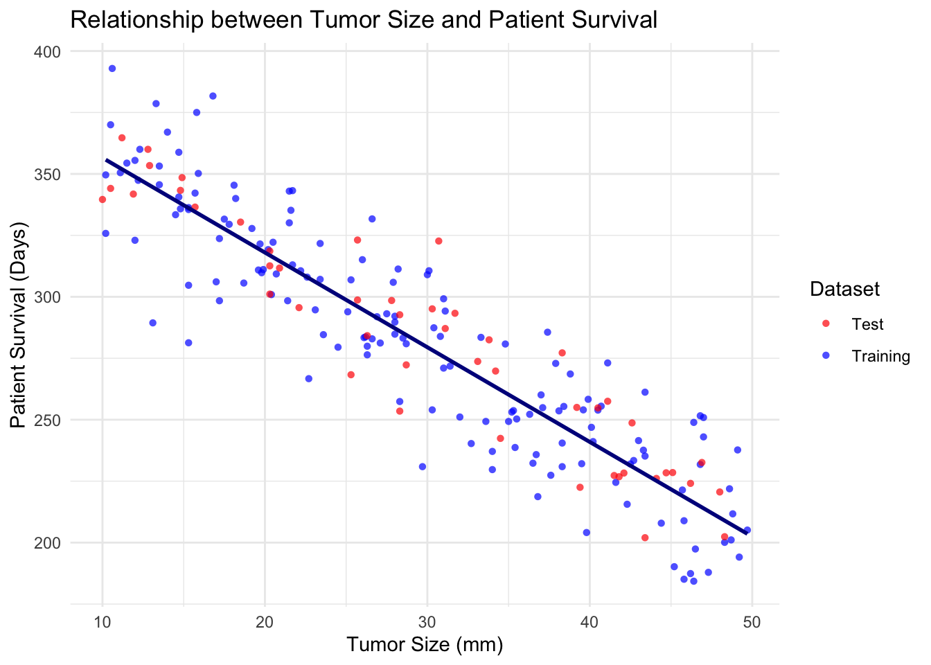
| Version | Author | Date |
|---|---|---|
| 897778a | tkcaccia | 2024-09-16 |
Multivariate Linear Regression
Most real-life scenarios are characterised by multivariate or high-dimensional features where more than one independent variable influences the target or dependent variable. Multi variate algorithms fit the model;
The mpg dataset from the ggplot2 package
can be used for multivariate regression. It includes information on car
attributes. we will choose some relevant attributes to predict
hwy, miles per gallon (MPG).
Step 1: Loading the dataset
# Load the dataset
library(ggplot2)
data(mpg)
df <- mpg
head(df)
# A tibble: 6 × 11
manufacturer model displ year cyl trans drv cty hwy fl class
<chr> <chr> <dbl> <int> <int> <chr> <chr> <int> <int> <chr> <chr>
1 audi a4 1.8 1999 4 auto(l5) f 18 29 p compa…
2 audi a4 1.8 1999 4 manual(m5) f 21 29 p compa…
3 audi a4 2 2008 4 manual(m6) f 20 31 p compa…
4 audi a4 2 2008 4 auto(av) f 21 30 p compa…
5 audi a4 2.8 1999 6 auto(l5) f 16 26 p compa…
6 audi a4 2.8 1999 6 manual(m5) f 18 26 p compa…We can choose predictors; displ - (engine displacement),
cyl - (number of cylinders), year - (year of
the car) and class - (type of car)
Step 2: Splitting and preparing the dataset
library(caret)

set.seed(30) # for reproducibility

# Split the data into training and testing sets
trainIndex <- createDataPartition(df$hwy, p = 0.75, list = FALSE)
trainData <- df[trainIndex, ]
testData <- df[-trainIndex, ]
Step 3: Fitting the model
model_mv <- lm(hwy ~ displ + cyl + year + class, data = trainData)
summary(model_mv)
Call:
lm(formula = hwy ~ displ + cyl + year + class, data = trainData)

Residuals:
    Min      1Q  Median      3Q     Max
-5.1700 -1.5322 -0.1473  1.0249 15.1030

Coefficients:
                  Estimate Std. Error t value Pr(>|t|)
(Intercept)     -183.14115   91.73394  -1.996 0.047511 *
displ             -1.06300    0.52272  -2.034 0.043576 *
cyl               -1.11663    0.36516  -3.058 0.002596 **
year               0.11135    0.04593   2.424 0.016399 *
classcompact      -4.06888    1.94849  -2.088 0.038295 *
classmidsize      -3.82081    1.89582  -2.015 0.045468 *
classminivan      -6.82814    1.98819  -3.434 0.000749 ***
classpickup      -10.55172    1.76709  -5.971 1.38e-08 ***
classsubcompact   -3.29990    1.90675  -1.731 0.085364 .
classsuv          -9.35511    1.70649  -5.482 1.53e-07 ***
---
Signif. codes:  0 '***' 0.001 '**' 0.01 '*' 0.05 '.' 0.1 ' ' 1

Residual standard error: 2.7 on 167 degrees of freedom
Multiple R-squared:  0.8091,    Adjusted R-squared:  0.7989
F-statistic: 78.67 on 9 and 167 DF,  p-value: < 2.2e-16
Step 4: Evaluating the model
test_predictions_mv <- predict(model_mv, newdata = testData)
mae <- MAE(test_predictions_mv, testData$hwy)
rmse <- RMSE(test_predictions_mv, testData$hwy)
r2_score <- summary(model)$r.squared

cat('MAE on test set (in days): ', mae, "\n",
  'RMSE on test set (in days): ', rmse, "\n",
  'R-Squared Score: ', r2_score)
MAE on test set (in days): 1.804035
RMSE on test set (in days): 2.325899
R-Squared Score: 0.820814Classification
Logistic Regression (LR)
logistic regression is classification algorithm used to predict a binary class label (for example, 0 or 1, cancer or no cancer).
LR has much in common with linear regression, the difference being
that linear regression is used to predict a
continuous target, whereas logistic regression is used to
predict a categorical target.
We can modify the iris dataset to demonstrate logistic
regression for binary classification by classifying whether a flower is
of “setosa” species or not.
Step 1: Data Preparation
Converting the iris data set into binary classification by creating a
variable Issetosa
data(iris)
head(iris)
Sepal.Length Sepal.Width Petal.Length Petal.Width Species
1 5.1 3.5 1.4 0.2 setosa
2 4.9 3.0 1.4 0.2 setosa
3 4.7 3.2 1.3 0.2 setosa
4 4.6 3.1 1.5 0.2 setosa
5 5.0 3.6 1.4 0.2 setosa
6 5.4 3.9 1.7 0.4 setosairis$IsSetosa <- ifelse(iris$Species == "setosa", 1, 0)
head(iris) Sepal.Length Sepal.Width Petal.Length Petal.Width Species IsSetosa
1 5.1 3.5 1.4 0.2 setosa 1
2 4.9 3.0 1.4 0.2 setosa 1
3 4.7 3.2 1.3 0.2 setosa 1
4 4.6 3.1 1.5 0.2 setosa 1
5 5.0 3.6 1.4 0.2 setosa 1
6 5.4 3.9 1.7 0.4 setosa 1Step 2: Splitting the dataset
Split the dataset into training (75%) and test (25%) sets
library(caret)
set.seed(123) # for reproducibility

#
train_index <- createDataPartition(iris$IsSetosa, p = 0.75, list = FALSE)
train_data <- iris[train_index, ]
test_data <- iris[-train_index, ]
Step 3: Fitting the logistic regression model
We shall predict IsSetosa using
Sepal.Length and Sepal.Width
model_lr <- glm(IsSetosa ~ Sepal.Length + Sepal.Width, data = train_data, family = binomial)

summary(model_lr)
Call:
glm(formula = IsSetosa ~ Sepal.Length + Sepal.Width, family = binomial,
    data = train_data)

Coefficients:
             Estimate Std. Error z value Pr(>|z|)
(Intercept)     442.8   144901.2   0.003    0.998
Sepal.Length   -165.6    51459.9  -0.003    0.997
Sepal.Width     139.8    51477.0   0.003    0.998

(Dispersion parameter for binomial family taken to be 1)

    Null deviance: 1.4431e+02  on 112  degrees of freedom
Residual deviance: 2.1029e-08  on 110  degrees of freedom
AIC: 6

Number of Fisher Scoring iterations: 25
Step 4: Making Predictions
# Make predictions on the training data
test_predictions <- predict(model_lr, newdata = test_data, type = "response")

# Convert the predicted probabilities to binary outcomes
predicted_class <- ifelse(test_predictions > 0.5, 1, 0)

predicted_class
1 2 3 5 11 18 19 28 33 36 48 49 55 56 57 58 59 61 62 65
1 1 1 1 1 1 1 1 1 1 1 1 0 0 0 0 0 0 0 0
66 70 77 83 84 94 95 98 100 105 111 113 116 125 131 135 141
0 0 0 0 0 0 0 0 0 0 0 0 0 0 0 0 0 Step 5: Evaluating the model
Confusion matrix
A confusion matrix is a 2×2 table that shows the predicted values from the model vs. the actual values from the test dataset.
It is a common way to evaluate the performance of a logistic regression model.
library(caret)

# Create a confusion matrix using caret
conf_matrix <- confusionMatrix(as.factor(predicted_class), as.factor(test_data$IsSetosa))
print(conf_matrix)
Confusion Matrix and Statistics
Reference
Prediction 0 1
0 25 0
1 0 12
Accuracy : 1
95% CI : (0.9051, 1)
No Information Rate : 0.6757
P-Value [Acc > NIR] : 5.016e-07
Kappa : 1
Mcnemar's Test P-Value : NA
Sensitivity : 1.0000
Specificity : 1.0000
Pos Pred Value : 1.0000
Neg Pred Value : 1.0000
Prevalence : 0.6757
Detection Rate : 0.6757
Detection Prevalence : 0.6757
Balanced Accuracy : 1.0000
'Positive' Class : 0
library(ggplot2)
library(reshape2)

# Convert confusion matrix to a dataframe
conf_matrix_df <- as.data.frame(conf_matrix$table)

# Create a heatmap using ggplot2
ggplot(data = conf_matrix_df, aes(x = Reference, y = Prediction, fill = Freq)) +
  geom_tile() +
  geom_text(aes(label = Freq), vjust = 1) +
  scale_fill_gradient(low = "white", high = "steelblue") +
  theme_minimal() +
  labs(title = "Confusion Matrix", x = "Actual", y = "Predicted")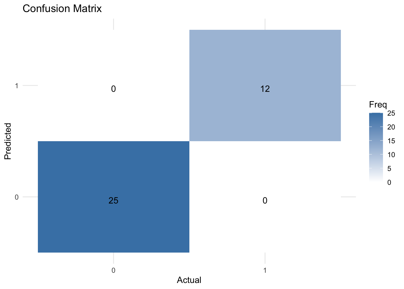
| Version | Author | Date |
|---|---|---|
| 897778a | tkcaccia | 2024-09-16 |
- Sensitivity: The “true positive rate” – the measure of how well the model correctly predicted positive cases.
- Specificity: The “true negative rate” – the measure of how well the model correctly predicted positive cases.
- Total miss-classification rate: The percentage of total incorrect classifications made by the model.
Receiver-operating characteristic curve (ROC)
The ROC curve is a visual representation of model performance across all thresholds.
The ROC curve is drawn by calculating the true positive rate (TPR) and false positive rate (FPR) at every possible threshold, then graphing TPR over FPR
Area under the curve (AUC)
The area under the ROC curve (AUC) represents the probability that the model, if given a randomly chosen positive and negative example, will rank the positive higher than the negative.
library(pROC)
# Create ROC curve
roc_curve <- roc(test_data$IsSetosa, test_predictions)

# Plot ROC curve
plot(roc_curve, main = "ROC Curve", col = "blue", lwd = 2)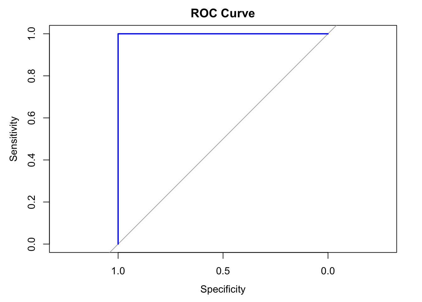
| Version | Author | Date |
|---|---|---|
| 897778a | tkcaccia | 2024-09-16 |
# Compute AUC
auc_value <- auc(roc_curve)
print(paste("AUC: ", round(auc_value, 4)))
[1] "AUC: 1"k-Nearest Neighbors (kNN)
K-nearest neighbors works by directly measuring the (Euclidean) distance between observations and inferring the class of unlabeled data from the class of its nearest neighbors.
Typically in machine learning, there are two clear steps, where one
first trains a model and then uses the model to predict new
outputs (class labels in this case). In the kNN, these two
steps are combined into a single function call to knn.
Lets draw a set of 50 random iris observations to train the model and predict the species of another set of 50 randomly chosen flowers. The knn function takes the training data, the new data (to be inferred) and the labels of the training data, and returns (by default) the predicted class.
set.seed(12L)
train <- sample(150, 50)
test <- sample(150, 50)
library("class")
knnres <- knn(iris[train, -5], iris[test, -5], iris$Species[train])
head(knnres)
[1] versicolor setosa versicolor setosa setosa setosa
Levels: setosa versicolor virginicaTree-based Methods
Tree-based methods are supervised learning algorithms that partition data into subsets based on feature values.
Types of Tree-based methods;
Decision trees: In these models where each internal node represents a feature test, each branch represents the outcome of the test, and each leaf node represents a class label or a continuous value
Ensemble Methods: These methods combine multiple decision trees to improve performance. Examples include; Random Forest model, boosting models (Xboost)
Decision Trees
Decision trees can be used as classification or regression algorithms.
Let us classify the species of iris flowers based on the features in the dataset.
Step 1: Loading Libraries and the dataset
#install.packages("rpart.plot")
#install.packages("randomForest")
library(caret)
library(rpart)
library(rpart.plot)
library(randomForest)

# Load the iris dataset
data(iris)
Step 2: Fitting the decision tree model
model_tree <- rpart(Species ~ ., data = iris, method = "class")Step 3: Plotting the decision tree
rpart.plot(model_tree, main = "Decision Tree for Iris Dataset")
| Version | Author | Date |
|---|---|---|
| 897778a | tkcaccia | 2024-09-16 |
Step 4: Making predictions and model evaluation
tree_predictions <- predict(model_tree, type = "class")
conf_matrix_tree <- confusionMatrix(tree_predictions, iris$Species)
print("Decision Tree Confusion Matrix: ")
[1] "Decision Tree Confusion Matrix: "print(conf_matrix_tree)Confusion Matrix and Statistics
Reference
Prediction setosa versicolor virginica
setosa 50 0 0
versicolor 0 49 5
virginica 0 1 45
Overall Statistics
Accuracy : 0.96
95% CI : (0.915, 0.9852)
No Information Rate : 0.3333
P-Value [Acc > NIR] : < 2.2e-16
Kappa : 0.94
Mcnemar's Test P-Value : NA
Statistics by Class:
Class: setosa Class: versicolor Class: virginica
Sensitivity 1.0000 0.9800 0.9000
Specificity 1.0000 0.9500 0.9900
Pos Pred Value 1.0000 0.9074 0.9783
Neg Pred Value 1.0000 0.9896 0.9519
Prevalence 0.3333 0.3333 0.3333
Detection Rate 0.3333 0.3267 0.3000
Detection Prevalence 0.3333 0.3600 0.3067
Balanced Accuracy 1.0000 0.9650 0.9450Random Forest Model
A random forest allows us to determine the most important predictors across the explanatory variables by generating many decision trees and then ranking the variables by importance.
Step 1: Fitting the random forest model
model_rf <- randomForest(Species ~ ., data = iris, ntree = 100)

# Print model summary
print(model_rf)
Call:
 randomForest(formula = Species ~ ., data = iris, ntree = 100)
               Type of random forest: classification
                     Number of trees: 100
No. of variables tried at each split: 2

        OOB estimate of  error rate: 6%
Confusion matrix:
           setosa versicolor virginica class.error
setosa         50          0         0        0.00
versicolor      0         47         3        0.06
virginica       0          6        44        0.12
Step 2: Making predictions and model evaluation
# Make predictions and evaluate
rf_predictions <- predict(model_rf)
conf_matrix_rf <- confusionMatrix(rf_predictions, iris$Species)
print("Random Forest Confusion Matrix:")
[1] "Random Forest Confusion Matrix:"print(conf_matrix_rf)Confusion Matrix and Statistics
Reference
Prediction setosa versicolor virginica
setosa 50 0 0
versicolor 0 47 6
virginica 0 3 44
Overall Statistics
Accuracy : 0.94
95% CI : (0.8892, 0.9722)
No Information Rate : 0.3333
P-Value [Acc > NIR] : < 2.2e-16
Kappa : 0.91
Mcnemar's Test P-Value : NA
Statistics by Class:
Class: setosa Class: versicolor Class: virginica
Sensitivity 1.0000 0.9400 0.8800
Specificity 1.0000 0.9400 0.9700
Pos Pred Value 1.0000 0.8868 0.9362
Neg Pred Value 1.0000 0.9691 0.9417
Prevalence 0.3333 0.3333 0.3333
Detection Rate 0.3333 0.3133 0.2933
Detection Prevalence 0.3333 0.3533 0.3133
Balanced Accuracy 1.0000 0.9400 0.92503 Getting Started
To load the package, enter the following instruction in your R session:
library("fastPLS")If this command terminates without any error messages, you can be sure that the package has been installed successfully. The fastPLS package is now ready for use.
The package includes both a user manual (this document) and a
reference manual (help pages for each function). To view the user
manual, enter vignette("fastPLS"). Help pages can be viewed
using the help command help(package="fastPLS").
Example using iris dataset
To load the package and dataset, input the following command in your R session:
library(fastPLS)
data(iris)
The iris dataset consists of 50 samples comprising of three different species:Setosa, Versicolor, and Virginica. These are classified as categorical variables. Four features were measured in centimeters (cm): the lengths and the widths of both sepals and petals. These features are used to determine the specie of the samples.
View the content of the dataset by using the command below:
head(iris)Select a random samples from the large dataset
ss=sample(150,15)Split the predictors and the response data
Xtrain=iris[-ss,-5]
Xtest=iris[ss,-5]
Ytrain=iris[-ss,5]
Ytest=iris[ss,5]
labels=iris[,5]
Perform pls on the dataset
z=pls(Xtrain,Ytrain,Xtest)Assign variable to the predicted and actual labels
predictions <- z$Ypred
actual_labels <- labels[ss]
Create a dataframe that shows the predicted and the actual label
results <- data.frame(Predicted = predictions, Actual= actual_labels)
results
V1 Actual
1 setosa setosa
2 virginica virginica
3 virginica versicolor
4 versicolor versicolor
5 setosa setosa
6 virginica virginica
7 versicolor virginica
8 versicolor versicolor
9 versicolor versicolor
10 versicolor versicolor
11 setosa setosa
12 versicolor virginica
13 setosa setosa
14 virginica versicolor
15 virginica versicolorConclusion
The table above gives a comparison of the predicted and actual label. This shows that the pls model was not efficient or accurate to predict some of the labels. This method is limited by the user inability to select the number of component to use, which affects the accuracy of the model
Choosing the number of component
Selecting the number of components when performing partial least square regression is crucial for achieving a good performance model.
Below is an example of how to input number of component for a model
    pp=pls(Xtrain,Ytrain,Xtest,ncomp = c(2,4))
    pp$Ypred
V1 V2
1 setosa setosa
2 virginica virginica
3 virginica virginica
4 versicolor versicolor
5 setosa setosa
6 virginica virginica
7 virginica versicolor
8 versicolor versicolor
9 versicolor versicolor
10 versicolor versicolor
11 setosa setosa
12 virginica versicolor
13 setosa setosa
14 versicolor virginica
15 virginica virginica pp=pls(Xtrain,Ytrain,Xtest,proj=TRUE)
plot(pp$Ttrain,col=Ytrain)
points(pp$Ttest,col=Ytest,pch=2)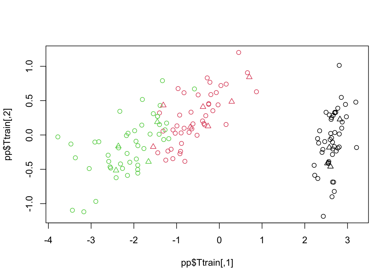
| Version | Author | Date |
|---|---|---|
| 5c88776 | tkcaccia | 2025-02-18 |
The graph above shows the PLS model performance to be able to project the Xtest (represented in triangles). The graph shows that the test points does not align well with the training cluster from the overlapping and the model is not efficient enough to distinguish the different groups.
Apart from the graphical result, different parameters can be used to assess the efficency of the model. Parameters such as Q2Y, R2Y and confusion matrix.
Q2Y:Measures the predictive power of the model on unseen/new data.If Q2Y>0.5,the model has good predictive ability, Q2Y>0.9 means excellent predictive power and Q2Y close to 0 or negative the model is poor at prediction.
Run the command below:
    pp=pls(Xtrain,Ytrain,Xtest,Ytest)
    pp$Q2Y
[1] -0.027485R2Y: Measures how well the model explains the response variable (Ytrain).R²Y close to 1 means a good fit while R²Y close to 0 represent model does not explain Y well.
Run the command below:
    pp=pls(Xtrain,Ytrain,fit=TRUE)
    pp$Yfit
ncomp=4
1 setosa
2 setosa
3 setosa
4 setosa
5 setosa
6 setosa
7 setosa
8 setosa
9 setosa
10 setosa
11 setosa
12 setosa
13 setosa
14 setosa
15 setosa
16 setosa
17 setosa
18 setosa
19 setosa
20 setosa
21 setosa
22 setosa
23 setosa
24 setosa
25 setosa
26 setosa
27 setosa
28 setosa
29 setosa
30 setosa
31 setosa
32 setosa
33 setosa
34 setosa
35 setosa
36 setosa
37 setosa
38 setosa
39 setosa
40 setosa
41 setosa
42 setosa
43 setosa
44 setosa
45 setosa
46 setosa
47 virginica
48 virginica
49 virginica
50 versicolor
51 versicolor
52 versicolor
53 virginica
54 versicolor
55 virginica
56 versicolor
57 virginica
58 versicolor
59 versicolor
60 virginica
61 virginica
62 versicolor
63 versicolor
64 versicolor
65 virginica
66 versicolor
67 versicolor
68 versicolor
69 versicolor
70 versicolor
71 virginica
72 versicolor
73 versicolor
74 versicolor
75 versicolor
76 virginica
77 virginica
78 virginica
79 versicolor
80 versicolor
81 versicolor
82 versicolor
83 versicolor
84 versicolor
85 versicolor
86 versicolor
87 versicolor
88 versicolor
89 versicolor
90 virginica
91 virginica
92 virginica
93 virginica
94 virginica
95 virginica
96 virginica
97 versicolor
98 versicolor
99 virginica
100 virginica
101 virginica
102 virginica
103 virginica
104 virginica
105 virginica
106 virginica
107 virginica
108 versicolor
109 virginica
110 versicolor
111 virginica
112 virginica
113 virginica
114 virginica
115 virginica
116 virginica
117 versicolor
118 virginica
119 virginica
120 versicolor
121 virginica
122 virginica
123 virginica
124 virginica
125 virginica
126 virginica
127 virginica
128 virginica
129 virginica
130 virginica
131 virginica
132 virginica
133 virginica
134 virginica
135 virginica pp$R2Y [,1]
[1,] 0.6024956Number of components
The above result model was optimized using 2 components which was indicated as ncomp = c(2,4).
Selecting too few or too many components can lead to underfitting or overfitting, respectively.
A statistical model or a machine learning algorithm is said to have underfitting when a model is too simple to capture data complexities. It represents the inability of the model to learn the training data effectively result in poor performance both on the training and testing data
Overfitting occurs when a model algorithm fails to give prediction on new dataset however gives ideal prediction on training dataset.This occurs when the model has been over-trained on a single or specific dataset.
Cross Validation
Cross validation is a method used in machine learning to evaluate the performance of a model on test data.
The dataset used are split into multiple folds or subsets, one of the folds is used as validation set and the reminder subset are used to train the model.This process is repeated several times, with a different fold used as the validation set each time.Finally, the results from each validation step are averaged to provide a more reliable estimate of the model’s performance.
Cross validation technique is useful in machine learning algorithm to avoid overfitting.
Types of Cross-Validation

PLS Double Cross-Validation
Double cross-validation is an approach to model hyperparameter optimization and model selection that attempts to overcome the problem of overfitting the training dataset. This involves two stages, outer and inner cross-validation.
Outer cross-validation evaluates the overall performance of the model. The dataset is split multiple times(K-fold cross-validation) and each time, the model is trained and tested on a different subset.
Inner cross-validation performs hyperparameter tuning to identify and select optimal parameter used in training a machine learning model.The training set of the outer fold is further split into sub-folds and the model is trained multiple times using different parameters.

In the next step, we apply pls double cross-validation to iris dataset
pp=pls.double.cv(iris[,-5],(iris[,5]),ncomp=2:4)To assess the prediction ability of the model, a 10-fold cross-validation is conducted by generating splits with a ratio 1:9 of the data set, that is by removing 10% of samples prior to any step of the statistical analysis, including PLS component selection and scaling. Best number of component for PLS was carried out by means of 10-fold cross-validation on the remaining 90% selecting the best Q2y value. Permutation testing was undertaken to estimate the classification/regression performance of predictors.
Optimal number of PLS components
    pp=optim.pls.cv(iris[,-5],(iris[,5]),ncomp=2:4)
    pp$optim_comp
[,1]
[1,] 4Feature transformation
Is the process of modifying and converting input features of a data set by applying mathematical operations to improve the learning and prediction performance of ML models.
Transformation techniques include scaling, normalisation and logarithmisation, which deal with differences in scale and distribution between features, non-linearity and outliers.
Input features (variables) may have different units, e.g. kilometre, day, year, etc., and so the variables have different scales and probably different distributions which increases the learning difficulty of ML algorithms from the data.
Normalisation
A number of different normalization methods are provided in KODAMA:
“none”: no normalization method is applied.
“pqn”: the Probabilistic Quotient Normalization is computed as described in Dieterle, et al. (2006).
“sum”: samples are normalized to the sum of the absolute value of all variables for a given sample.
“median”: samples are normalized to the median value of all variables for a given sample.
“sqrt”: samples are normalized to the root of the sum of the squared value of all variables for a given sample.
library(KODAMA)

data(MetRef)
u=MetRef$data;
u=u[,-which(colSums(u)==0)]
u=normalization(u)$newXtrain
class=as.numeric(as.factor(MetRef$gender))
cc=pca(u)
plot(cc$x,pch=21,bg=class)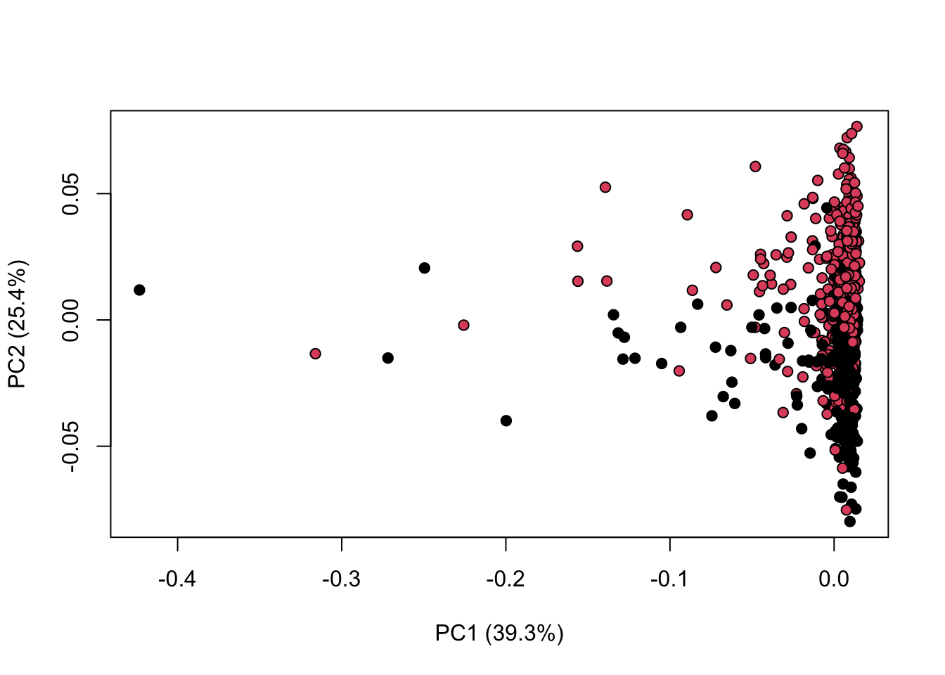
| Version | Author | Date |
|---|---|---|
| 897778a | tkcaccia | 2024-09-16 |
Scaling and Standardisation
A number of different scaling methods are provided in KODAMA:
“
none”: no scaling method is applied.“
centering”: centers the mean to zero.“
autoscaling”: centers the mean to zero and scales data by dividing each variable by the variance.“
rangescaling”: centers the mean to zero and scales data by dividing each variable by the difference between the minimum and the maximum value.“
paretoscaling”: centers the mean to zero and scales data by dividing each variable by the square root of the standard deviation. Unit scaling divides each variable by the standard deviation so that each variance equal to 1.
library(KODAMA)
data(MetRef)
u=MetRef$data;
u=u[,-which(colSums(u)==0)]
u=scaling(u)$newXtrain
class=as.numeric(as.factor(MetRef$gender))
cc=pca(u)
plot(cc$x,pch=21,bg=class,xlab=cc$txt[1],ylab=cc$txt[2])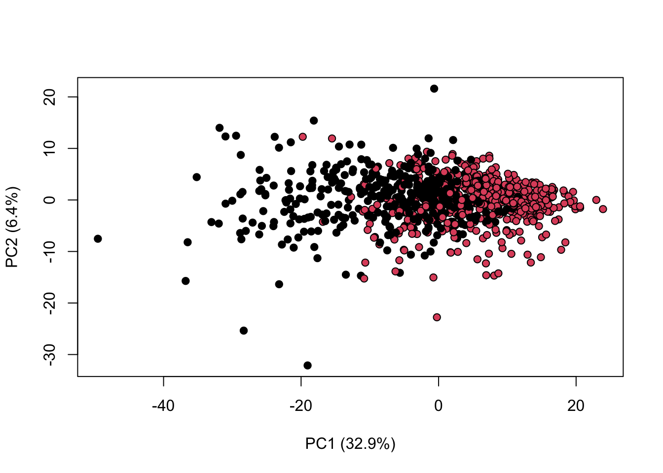
| Version | Author | Date |
|---|---|---|
| 897778a | tkcaccia | 2024-09-16 |
We can combine both normalisation and scaling to see the difference in the output
library(KODAMA)
data(MetRef)
u=MetRef$data;
u=u[,-which(colSums(u)==0)]
u=normalization(u)$newXtrain
u=scaling(u)$newXtrain
class=as.numeric(as.factor(MetRef$gender))
cc=pca(u)
plot(cc$x,pch=21,bg=class,xlab=cc$txt[1],ylab=cc$txt[2])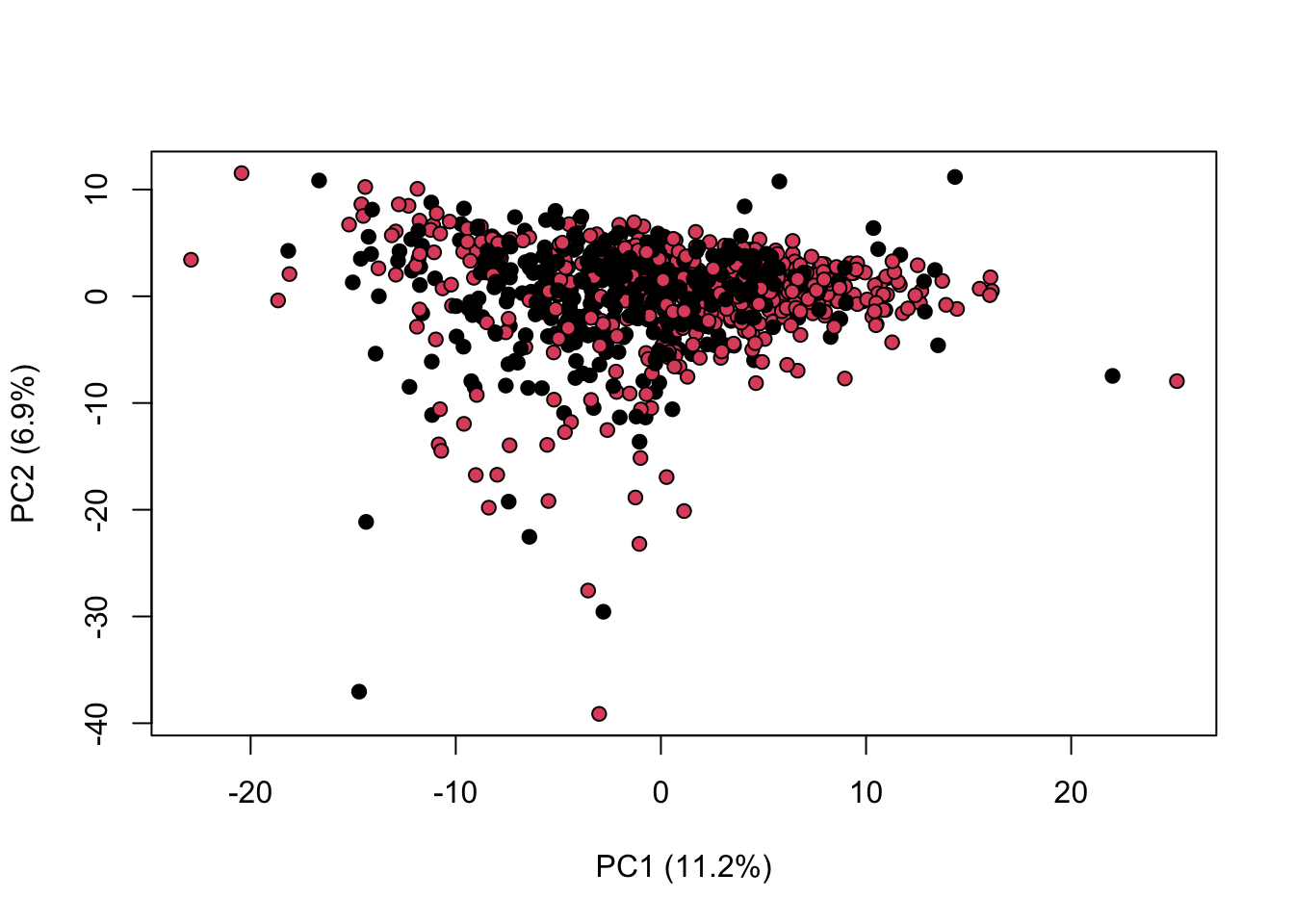
| Version | Author | Date |
|---|---|---|
| 897778a | tkcaccia | 2024-09-16 |
sessionInfo()R version 4.3.3 (2024-02-29)
Platform: aarch64-apple-darwin20 (64-bit)
Running under: macOS Sonoma 14.5
Matrix products: default
BLAS: /Library/Frameworks/R.framework/Versions/4.3-arm64/Resources/lib/libRblas.0.dylib
LAPACK: /Library/Frameworks/R.framework/Versions/4.3-arm64/Resources/lib/libRlapack.dylib; LAPACK version 3.11.0
locale:
[1] en_US.UTF-8/en_US.UTF-8/en_US.UTF-8/C/en_US.UTF-8/en_US.UTF-8
time zone: Africa/Johannesburg
tzcode source: internal
attached base packages:
[1] stats graphics grDevices utils datasets methods base
other attached packages:
[1] KODAMA_3.0 umap_0.2.10.0 Rtsne_0.17
[4] minerva_1.5.10 fastPLS_0.2 Matrix_1.6-5
[7] randomForest_4.7-1.2 rpart.plot_3.1.2 rpart_4.1.24
[10] class_7.3-23 pROC_1.18.5 reshape2_1.4.4
[13] caret_7.0-1 lattice_0.22-6 ggplot2_3.5.2
[16] workflowr_1.7.1
loaded via a namespace (and not attached):
[1] tidyselect_1.2.1 timeDate_4041.110 dplyr_1.1.4
[4] farver_2.1.2 fastmap_1.2.0 promises_1.3.2
[7] digest_0.6.37 timechange_0.3.0 lifecycle_1.0.4
[10] survival_3.8-3 processx_3.8.6 magrittr_2.0.3
[13] compiler_4.3.3 rlang_1.1.6 sass_0.4.9
[16] tools_4.3.3 utf8_1.2.6 yaml_2.3.10
[19] data.table_1.17.8 knitr_1.50 askpass_1.2.1
[22] labeling_0.4.3 reticulate_1.42.0 plyr_1.8.9
[25] RColorBrewer_1.1-3 withr_3.0.2 purrr_1.0.4
[28] nnet_7.3-20 grid_4.3.3 stats4_4.3.3
[31] git2r_0.36.2 e1071_1.7-16 future_1.34.0
[34] globals_0.16.3 scales_1.4.0 iterators_1.0.14
[37] MASS_7.3-60.0.1 cli_3.6.5 rmarkdown_2.29
[40] generics_0.1.4 RSpectra_0.16-2 rstudioapi_0.17.1
[43] future.apply_1.11.3 httr_1.4.7 proxy_0.4-27
[46] cachem_1.1.0 stringr_1.5.1 splines_4.3.3
[49] parallel_4.3.3 vctrs_0.6.5 hardhat_1.4.1
[52] jsonlite_2.0.0 callr_3.7.6 listenv_0.9.1
[55] foreach_1.5.2 gower_1.0.2 jquerylib_0.1.4
[58] recipes_1.2.1 glue_1.8.0 parallelly_1.43.0
[61] codetools_0.2-20 ps_1.9.0 lubridate_1.9.4
[64] stringi_1.8.7 gtable_0.3.6 later_1.4.1
[67] tibble_3.3.0 pillar_1.11.0 htmltools_0.5.8.1
[70] openssl_2.3.2 ipred_0.9-15 lava_1.8.1
[73] R6_2.6.1 rprojroot_2.0.4 evaluate_1.0.3
[76] png_0.1-8 httpuv_1.6.15 bslib_0.9.0
[79] Rcpp_1.1.0 nlme_3.1-168 prodlim_2024.06.25
[82] mgcv_1.9-1 whisker_0.4.1 xfun_0.52
[85] fs_1.6.6 getPass_0.2-4 pkgconfig_2.0.3
[88] ModelMetrics_1.2.2.2