Introduction
Stefano Cacciatore
August 13, 2025
Last updated: 2025-08-13
Checks: 7 0
Knit directory: Tutorials/
This reproducible R Markdown analysis was created with workflowr (version 1.7.1). The Checks tab describes the reproducibility checks that were applied when the results were created. The Past versions tab lists the development history.
Great! Since the R Markdown file has been committed to the Git repository, you know the exact version of the code that produced these results.
Great job! The global environment was empty. Objects defined in the global environment can affect the analysis in your R Markdown file in unknown ways. For reproduciblity it’s best to always run the code in an empty environment.
The command set.seed(20240905) was run prior to running
the code in the R Markdown file. Setting a seed ensures that any results
that rely on randomness, e.g. subsampling or permutations, are
reproducible.
Great job! Recording the operating system, R version, and package versions is critical for reproducibility.
Nice! There were no cached chunks for this analysis, so you can be confident that you successfully produced the results during this run.
Great job! Using relative paths to the files within your workflowr project makes it easier to run your code on other machines.
Great! You are using Git for version control. Tracking code development and connecting the code version to the results is critical for reproducibility.
The results in this page were generated with repository version cd0328c. See the Past versions tab to see a history of the changes made to the R Markdown and HTML files.
Note that you need to be careful to ensure that all relevant files for
the analysis have been committed to Git prior to generating the results
(you can use wflow_publish or
wflow_git_commit). workflowr only checks the R Markdown
file, but you know if there are other scripts or data files that it
depends on. Below is the status of the Git repository when the results
were generated:
Ignored files:
    Ignored:    .DS_Store
    Ignored:    .RData
    Ignored:    .Rhistory
    Ignored:    data/.DS_Store

Unstaged changes:
    Modified:   output/Table.csv
Note that any generated files, e.g. HTML, png, CSS, etc., are not included in this status report because it is ok for generated content to have uncommitted changes.
These are the previous versions of the repository in which changes were
made to the R Markdown (analysis/Introduction.Rmd) and HTML
(docs/Introduction.html) files. If you’ve configured a
remote Git repository (see ?wflow_git_remote), click on the
hyperlinks in the table below to view the files as they were in that
past version.
| File | Version | Author | Date | Message |
|---|---|---|---|---|
| html | 9cf9cd7 | tkcaccia | 2025-08-13 | Build site. |
| html | 90b4df3 | tkcaccia | 2025-08-13 | Build site. |
| html | 36cba68 | tkcaccia | 2025-08-13 | Build site. |
| html | cbadb19 | tkcaccia | 2025-08-13 | Build site. |
| html | 5c88776 | tkcaccia | 2025-02-18 | Build site. |
| html | 5baa04e | tkcaccia | 2025-02-17 | Build site. |
| html | f26aafb | tkcaccia | 2025-02-17 | Build site. |
| Rmd | 012feeb | tkcaccia | 2025-02-17 | Start my new project |
| html | 1ce3cb4 | tkcaccia | 2025-02-16 | Build site. |
| html | 681ec51 | tkcaccia | 2025-02-16 | Build site. |
| Rmd | 39864ea | tkcaccia | 2025-02-16 | Start my new project |
| html | 9558051 | tkcaccia | 2024-09-18 | update |
| html | a7f82c5 | tkcaccia | 2024-09-18 | Build site. |
| html | a6eff7d | tkcaccia | 2024-09-16 | updates |
| html | 83f8d4e | tkcaccia | 2024-09-16 | Build site. |
| Rmd | 25c1d18 | tkcaccia | 2024-09-16 | Start my new project |
| html | 159190a | tkcaccia | 2024-09-16 | Build site. |
| Rmd | dff6a04 | tkcaccia | 2024-09-16 | Start my new project |
| html | 6d23cdb | tkcaccia | 2024-09-16 | Build site. |
| html | 6301d0a | tkcaccia | 2024-09-16 | Build site. |
| html | 897778a | tkcaccia | 2024-09-16 | Build site. |
| html | 1a34734 | tkcaccia | 2024-09-16 | Build site. |
| html | 5033c12 | tkcaccia | 2024-09-16 | Build site. |
| Rmd | e9cf751 | tkcaccia | 2024-09-16 | Start my new project |
Basics in R
Open RStudio and take a few minutes to explore each pane and its functionality.
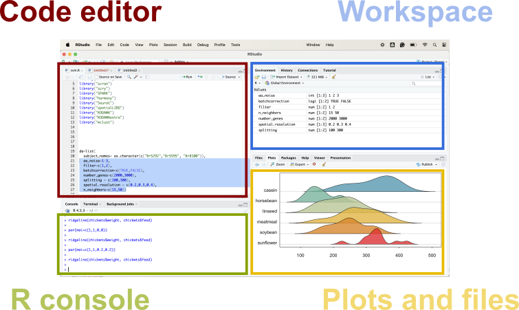
1. Familiarize with the RStudio Interface
In this section, we’ll get to know the RStudio interface and understand its different components:
Layout: The RStudio interface consists of several panes that help you manage your workflow efficiently.
Panes: These include the Source Pane, Console, Environment/History Pane, and the Files/Plots/Packages/Help/Viewer Pane.
Console: The Console is where you can directly execute R commands.
Script Editor: The Script Editor is used for writing and editing scripts, which can be executed in parts or as a whole.
Environment: The Environment Pane shows all the objects (data, functions, etc.) that you’ve created during your session.
2. Basic R Operations
Let’s start by performing some basic operations in R:
Arithmetic:
- addition, subtraction, multiplication, division etc.
# Basic Arithmetic
5 + 3 # Sum
[1] 85 - 3 # Difference[1] 25 * 3 # Product[1] 155 / 3 # Quotient[1] 1.6666675 ^ 3 # Exponent[1] 1255 %% 3 # Remainder from division[1] 2Variable Assignment:
- You can assign values to variables for reuse.
# Variable Assignment
x <- 10
y <- 20
z <- x + y # x and y are now saved in your environment for reuse
z
[1] 30Data Types: - Numeric, Character, Boolean, Integer, and Double
# 6 = numeric
# "c" = character
# -5 = integer
# TRUE = boolean
Data Formats:
vectors,
lists,
data frames
# Vectors = arrays of data elements each of the SAME TYPE.
vec <- c(1, 2, 3, 4, 5)
vec
[1] 1 2 3 4 5# Lists = can contain many items that (can have different types of data like numbers characters and also could contain stored vectors or data frames.)
lst <- list(name = "John", age = 25)
lst$name
[1] "John"
$age
[1] 25# Data Frames = tabular (2-dimensional) data structure that can store values of any data type.
df <- data.frame(Name = c("Alice", "Bob"), Age = c(25, 30))
df Name Age
1 Alice 25
2 Bob 303. Functions in R
Understanding and creating functions is fundamental in R:
- Functions are reusable blocks of code that perform a specific task.
Creating Simple Functions: Here’s how you can create a simple function in R.
# Creating a Function
add_numbers <- function(a, b) {
  return(a + b)  # takes two arguments (a and b) and returns their sum.
}

# Using the Function: Here we are calling the function 'add_numbers' with 10 and 15 as inputs.
add_numbers(10, 15)
[1] 254. Installing and loading Packages:
R packages are collections of functions and datasets developed by the R community:
There are pre-loaded packages in Rstudio that can be used and called without installation (e.g., dplyr)
CRAN: CRAN (Comprehensive R Archive Network) is the main repository for R packages.
Installing and Loading Packages: To use additional functions, you might need to install and load packages.
# Installing a Package (Uncomment the line below if the package has been loaded previously)
install.packages("ggplot2")
Installing package into '/Users/stefano/Library/R/arm64/4.3/library'
(as 'lib' is unspecified)
The downloaded binary packages are in
    /var/folders/p9/7vjxs6dd7p70vybzdhy_0hw00000gn/T//RtmpY9oKSn/downloaded_packages
# Loading the package "ggplot" a data visualtion package we will use later in the course:
library(ggplot2) # no quotations needed when loading a package from your library5. Saving
- I have stored a data frame (with example data not shown) named “df”
# Can store columns of different data types

city <- c("Cairo", "Kinshasa", "Lagos", "Luanda", "Dar es Salaam", "Khartoum",
          "Johannesburg", "Abidjan", "Addis Ababa", "Nairobi", "Yaoundé",
          "Casablanca", "Antananarivo", "Kampala", "Kumasi" , "Dakar",
          "Ouagadougou", "Lusaka", "Algiers", "Bamako", "Brazzaville",
          "Mogadishu", "Tunis", "Conakry", "Lomé", "Matola", "Monrovia",
          "Harare", "N'Djamena", "Nouakchott", "Niamey", "Freetown",
          "Lilongwe", "Kigali", "Abomey-Calavi", "Tripoli", "Bujumbura",
          "Asmara", "Bangui", "Libreville")

abb <- c("CA", "KI", "LA", "LU", "DS", "KH", "JO", "AB", "AD", "NA", "YA",
         "CB", "AN", "KA", "KU", "DA", "OU", "LS", "AL", "BA", "BR", "MO",
         "TU", "CO", "LO", "MA", "MN", "HA", "ND", "NO", "NI", "FR", "LI",
         "KG", "AC", "TR", "BU", "AS", "BG", "LB")

region <- c("North", "Central", "Central", "South", "South", "North",
            "South", "Central", "Central", "Central", "Central",
            "North", "South", "Central", "Central", "Central",
            "Central", "South", "North", "North", "South",
            "Central", "North", "Central", "Central", "South",
            "Central", "South", "North", "North", "North",
            "Central", "South", "Central", "Central", "North",
            "South", "Central", "Central", "Central")

region <- factor(region, levels = c("North", "Central" , "South"))

population <- c(22183200, 16315534, 15387639, 8952496, 7404689,
         6160327, 6065354, 5515790, 5227794, 5118844,
         4336670, 3840396, 3699900, 3651919, 3630326,
         3326001, 3055788, 3041789, 2853959, 2816943,
         2552813, 2497463, 2435961, 2048525, 1925517,
         1796872, 1622582, 1557740, 1532588, 1431539,
         1383909, 1272145, 1222325, 1208296, 1188736,
         1175830, 1139265, 1034872, 933176, 856854)

total <- c(125700, 80500, 66900, 51700, 36400, 45700, 31000,
           37600, 41300, 28600, 24600, 25000, 9300, 11800,
           14200, 23200, 21900, 32100, 29300, 9700, 5300,
           6500, 13500, 20700, 35100, 11600, 3600, 11100,
           9700, 2100, 12000, 9300, 6300, 2200, 8400,
           6700, 2700, 3200,1200, 700)
df <- data.frame(city, abb, region, population, total)
head(df) # shows the first 'n' rows city abb region population total
1 Cairo CA North 22183200 125700
2 Kinshasa KI Central 16315534 80500
3 Lagos LA Central 15387639 66900
4 Luanda LU South 8952496 51700
5 Dar es Salaam DS South 7404689 36400
6 Khartoum KH North 6160327 45700write.csv(df,"output/data.csv")6. Importing External Data:
Data analysis often involves importing data from external files:
R can read data from various formats like CSV, Excel, etc.
It is important to pay attention to the extension the file uses (e.g., csv = comman seperated values)
# Reading CSV Files:
df <- read.csv("output/data.csv")

# Reading Excel Files (requires the readxl package)
install.packages("readxl")
Installing package into '/Users/stefano/Library/R/arm64/4.3/library'
(as 'lib' is unspecified)
The downloaded binary packages are in
    /var/folders/p9/7vjxs6dd7p70vybzdhy_0hw00000gn/T//RtmpY9oKSn/downloaded_packages
library(readxl)
# df_excel <- read_excel("path/to/your/file.xlsx")7. Indexing:
- Indexing is the process of selecting elements using their indices (i.e., positions in the data format)
Indexing ROWS and COLUMNS by POSITION:
# Select 1st Row:
first_row <- df[1, ]  # Selects the entire first row

# Select 2nd column:
second_column <- df[, 2]  # Selects the entire second column ('abb')

# Select the element in the 3rd row and 4th column:
specific_element <- df[3, 4]  # Selects the population of the third city ('Lagos')
Indexing Using COLUMN Names:
# Select the 'city' column:
city_column <- df$city  # Selects the 'city' column

# Select the first row using column names:
first_row_city_pop <- df[1, c("city", "population")]  # Selects the 'city' and 'pop' columns for the first row

# Logical Indexing:
large_cities <- df[df$pop > 10000000, ]  # Returns all rows where 'pop' is greater than 10 million
Indexing with dplyr:
# Using dplyr you can perform similar operations with clearer syntax:
library(dplyr)

# Select specific columns
selected_df <- df %>%
  select(city, population)  # Selects 'city' and 'pop' columns

# Filter rows based on a condition
filtered_df <- df %>%
  filter(population > 10000000)  # Filters for cities with population greater than 10 million
8. Data Manipulation Basics
Basic data manipulation is key to preparing data for analysis.
Overview of Data Classes: Learn about data frames, matrices, and lists.
Data Frames: Rectangular tables with rows and columns, where columns can be of different types.
Matrices: Rectangular tables with rows and columns, where all elements must be of the same type.
Lists: Collections of elements that can be of different types, including other lists.
# Creating a Matrix
matrix_example <- matrix(1:9, nrow = 3, byrow = TRUE)

# Creating a List
list_example <- list(
  numbers = 1:5,
  text = c("A", "B", "C"),
  data_frame = df
)- Subsetting Data: Extract subsets of data based on conditions.
# Extract cities with population greater than 10 million
large_cities <- df[df$population > 10000000, ]

# Extract cities in the 'South' region
south_cities <- df[df$region == "South", ]

# Select Specific Columns
city_population <- df[, c("city", "population")]- Basic Transformations: Perform simple data transformations such as adding new columns.
# Add a New Column: City Area (dummy data)
df$area <- c(606, 851, 1171, 300, 400)  # Example areas in square kilometers

# Modify Existing Column: Increase Population by 10%
df$population <- df$population * 1.10

# Using dplyr for Data Manipulation:

# Add a New Column: City Area
df <- df %>%
  mutate(rank = 1:40)

# Modify Existing Column: Increase Population by 10%
df <- df %>%
  mutate(population = population * 1.10)

# Filter: Cities in the 'South' Region
south_cities_dplyr <- df %>%
  filter(region == "South")

# Select Specific Columns
city_population_dplyr <- df %>%
  select(city, population)
Exercise: :
a. Data Classes: Extract the population of the 3rd city from the df data frame.
b. Subsetting Data -> Extract the elements from matrix_example that are greater than 5.
c. Basic Transformations: Add a new column area to df with values 500, 600, 700, 800, 900.
Answer
# 7a:
df[3, "population"]
[1] 18619043# 7b:
matrix_example[matrix_example > 5][1] 7 8 6 9# 7c:
df$area <- c(500, 600, 700, 800, 900)
head(df) X city abb region population total area rank
1 1 Cairo CA North 26841672 125700 500 1
2 2 Kinshasa KI Central 19741796 80500 600 2
3 3 Lagos LA Central 18619043 66900 700 3
4 4 Luanda LU South 10832520 51700 800 4
5 5 Dar es Salaam DS South 8959674 36400 900 5
6 6 Khartoum KH North 7453996 45700 500 6
sessionInfo()R version 4.3.3 (2024-02-29)
Platform: aarch64-apple-darwin20 (64-bit)
Running under: macOS Sonoma 14.5
Matrix products: default
BLAS: /Library/Frameworks/R.framework/Versions/4.3-arm64/Resources/lib/libRblas.0.dylib
LAPACK: /Library/Frameworks/R.framework/Versions/4.3-arm64/Resources/lib/libRlapack.dylib; LAPACK version 3.11.0
locale:
[1] en_US.UTF-8/en_US.UTF-8/en_US.UTF-8/C/en_US.UTF-8/en_US.UTF-8
time zone: Africa/Johannesburg
tzcode source: internal
attached base packages:
[1] stats graphics grDevices utils datasets methods base
other attached packages:
[1] dplyr_1.1.4 readxl_1.4.5 ggplot2_3.5.2 workflowr_1.7.1
loaded via a namespace (and not attached):
[1] gtable_0.3.6 jsonlite_2.0.0 compiler_4.3.3 promises_1.3.2
[5] tidyselect_1.2.1 Rcpp_1.1.0 stringr_1.5.1 git2r_0.36.2
[9] callr_3.7.6 later_1.4.1 jquerylib_0.1.4 scales_1.4.0
[13] yaml_2.3.10 fastmap_1.2.0 R6_2.6.1 generics_0.1.4
[17] knitr_1.50 tibble_3.3.0 rprojroot_2.0.4 RColorBrewer_1.1-3
[21] bslib_0.9.0 pillar_1.11.0 rlang_1.1.6 cachem_1.1.0
[25] stringi_1.8.7 httpuv_1.6.15 xfun_0.52 getPass_0.2-4
[29] fs_1.6.6 sass_0.4.9 cli_3.6.5 withr_3.0.2
[33] magrittr_2.0.3 ps_1.9.0 digest_0.6.37 grid_4.3.3
[37] processx_3.8.6 rstudioapi_0.17.1 lifecycle_1.0.4 vctrs_0.6.5
[41] evaluate_1.0.3 glue_1.8.0 cellranger_1.1.0 farver_2.1.2
[45] whisker_0.4.1 rmarkdown_2.29 httr_1.4.7 tools_4.3.3
[49] pkgconfig_2.0.3 htmltools_0.5.8.1