FiberMargin: Complete User Guide

Purpose and input contract

FiberMargin repairs a categorical field from spatial coordinates and the observed labels alone. It does not use expression values, image intensities, logits, probabilities, clean anchors, or reference labels during repair.

There are two fixed computational routes:

Multiclass fields use the two-sided path-enclosure operator.
Binary fields use a distinct fixed nearest-neighbour ballot specialization.

The package accepts irregular 2D or 3D coordinates through refine_spatial_labels() and regular pixel or voxel arrays through clean_categorical_mask(). Multiple specimens can be supplied in one call and are always processed independently.

The package exports 14 functions:

api <- data.frame(
  Function = c(
    "refine_spatial_labels", "clean_categorical_mask",
    "corrupt_categorical_mask", "evaluate_mask_cleaning",
    "spatial_benchmark", "evaluate_spatial_refinement",
    "benchmark_spatial_refiners", "simulate_spatial_clusters",
    "simulate_spatial_domains", "simulate_complex_spatial_domains",
    "simulate_gradient_regions", "simulate_volumetric_domains",
    "available_spatial_benchmarks", "load_spatial_benchmark"
  ),
  Purpose = c(
    "Refine labels at irregular 2D/3D coordinates",
    "Clean a categorical matrix or 3D array",
    "Generate reproducible mask errors",
    "Score a cleaned mask",
    "Validate and package a benchmark",
    "Score coordinate-indexed refinement",
    "Run identical inputs through multiple methods",
    "Simulate separated Gaussian-like clusters",
    "Simulate structured 2D or curved-layer 3D domains",
    "Simulate held-out complex geometries",
    "Simulate the A-B-C gradient design",
    "Simulate variable-density 3D domains",
    "List real-data availability and licensing",
    "Load a bundled frozen real-data scenario"
  ),
  stringsAsFactors = FALSE
)
knitr::kable(api)

Function	Purpose
refine_spatial_labels	Refine labels at irregular 2D/3D coordinates
clean_categorical_mask	Clean a categorical matrix or 3D array
corrupt_categorical_mask	Generate reproducible mask errors
evaluate_mask_cleaning	Score a cleaned mask
spatial_benchmark	Validate and package a benchmark
evaluate_spatial_refinement	Score coordinate-indexed refinement
benchmark_spatial_refiners	Run identical inputs through multiple methods
simulate_spatial_clusters	Simulate separated Gaussian-like clusters
simulate_spatial_domains	Simulate structured 2D or curved-layer 3D domains
simulate_complex_spatial_domains	Simulate held-out complex geometries
simulate_gradient_regions	Simulate the A-B-C gradient design
simulate_volumetric_domains	Simulate variable-density 3D domains
available_spatial_benchmarks	List real-data availability and licensing
load_spatial_benchmark	Load a bundled frozen real-data scenario

Quick start

The gradient simulator creates four ordered areas with reference classes A, B, B, and C. Its observed labels contain controlled minority mixtures.

gradient <- simulate_gradient_regions(
  n = 1200L,
  minority = 0.10,
  dimensions = 2L,
  samples = 2L,
  density_profile = "moderate",
  seed = 12L
)

refined_gradient <- refine_spatial_labels(
  xy = gradient$xy,
  labels = gradient$labels,
  samples = gradient$samples,
  workers = 1L
)

gradient_metrics <- evaluate_spatial_refinement(
  truth = gradient$truth,
  initial = gradient$labels,
  refined = refined_gradient,
  boundary = gradient$boundary,
  regions = gradient$area,
  sparse = gradient$sparse,
  method = "FiberMargin"
)

gradient_metrics[, c(
  "method", "initial_accuracy", "accuracy", "ari",
  "correction_recall", "damage_rate"
)]
#>        method initial_accuracy accuracy       ari correction_recall damage_rate
#> 1 FiberMargin              0.9     0.98 0.9327002               0.9  0.01111111

old_par <- graphics::par(no.readonly = TRUE)
graphics::par(mfrow = c(1, 3), mar = c(3, 3, 2, 1))
plot_field(gradient$xy, gradient$truth, "Reference", cex = 0.35)
plot_field(gradient$xy, gradient$labels, "Observed", cex = 0.35)
plot_field(gradient$xy, refined_gradient, "FiberMargin", cex = 0.35)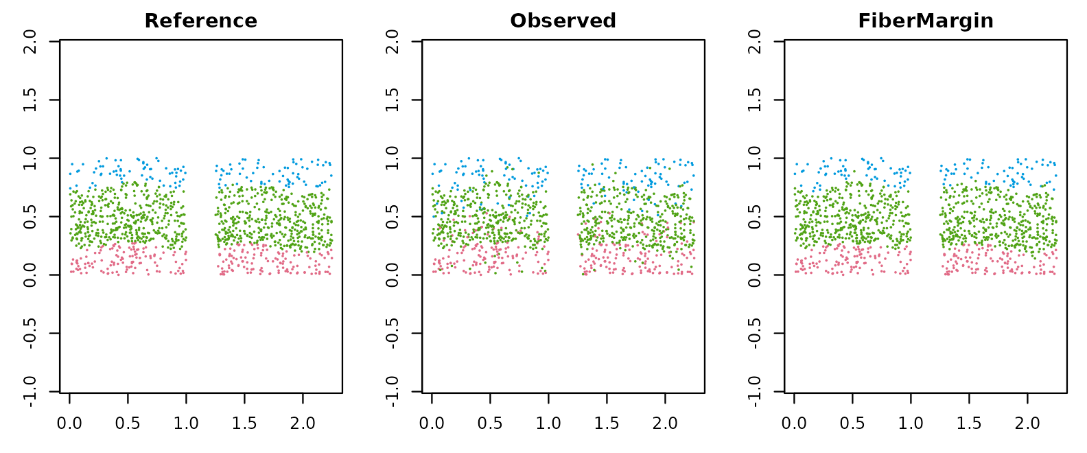

graphics::par(old_par)

Refine irregular coordinates

`refine_spatial_labels()`

refine_spatial_labels(xy, labels, samples = NULL, workers = NULL)

xy must be a finite numeric matrix with two or three columns. labels must contain one non-missing categorical value per row. samples is optional and defines independent coordinate systems. Integer, character, and factor specimen identifiers are accepted. workers = NULL uses a conservative automatic CPU budget; set a positive integer for an explicit total budget.

Effective dimensionality is determined separately within every specimen. Zero-range axes are removed before refinement. At least two varying axes must remain, so constant z reduces a three-column specimen to 2D while variable z remains part of a genuine 3D analysis.

The output is a factor with the input levels and row names. Seven pointwise audit attributes are attached:

diagnostic_names <- c(
  "candidate", "margin_score", "required", "repair_margin",
  "atlas_dispersion", "isolation", "changed"
)

diagnostics <- data.frame(
  observed = head(as.character(gradient$labels), 8L),
  refined = head(as.character(refined_gradient), 8L),
  candidate = head(as.character(attr(refined_gradient, "candidate")), 8L),
  margin_score = head(attr(refined_gradient, "margin_score"), 8L),
  required = head(attr(refined_gradient, "required"), 8L),
  repair_margin = head(attr(refined_gradient, "repair_margin"), 8L),
  changed = head(attr(refined_gradient, "changed"), 8L)
)
diagnostics
#>       observed refined candidate margin_score   required repair_margin changed
#> spot1        C       B         B    0.7351437 0.06036058     0.6747831    TRUE
#> spot2        B       B         B    0.0000000 0.00000000     0.0000000   FALSE
#> spot3        A       A         A    0.0000000 0.00000000     0.0000000   FALSE
#> spot4        B       B         B    0.0000000 0.00000000     0.0000000   FALSE
#> spot5        A       A         A    0.0000000 0.00000000     0.0000000   FALSE
#> spot6        A       A         A    0.0000000 0.00000000     0.0000000   FALSE
#> spot7        B       B         B    0.0000000 0.00000000     0.0000000   FALSE
#> spot8        B       B         B    0.0000000 0.00000000     0.0000000   FALSE

setdiff(diagnostic_names, names(attributes(refined_gradient)))
#> character(0)

candidate is the locally preferred class. margin_score is its support contrast, required is the local admission barrier, and repair_margin is margin_score - required. These are deterministic scores, not calibrated probabilities. atlas_dispersion describes disagreement across path charts, isolation protects locally isolated observations, and changed identifies accepted edits.

Eight summary attributes provide a specimen-level audit:

summary_names <- c(
  "workers", "dimensions_used", "labels_changed", "changed_fraction",
  "classes_before", "classes_after", "removed_classes", "sample_sizes"
)
lapply(summary_names, function(name) attr(refined_gradient, name))
#> [[1]]
#> [1] 1
#> 
#> [[2]]
#> 1 2 
#> 2 2 
#> 
#> [[3]]
#>  1  2 
#> 61 59 
#> 
#> [[4]]
#>          1          2 
#> 0.10166667 0.09833333 
#> 
#> [[5]]
#> [[5]]$`1`
#> [1] "A" "B" "C"
#> 
#> [[5]]$`2`
#> [1] "A" "B" "C"
#> 
#> 
#> [[6]]
#> [[6]]$`1`
#> [1] "A" "B" "C"
#> 
#> [[6]]$`2`
#> [1] "A" "B" "C"
#> 
#> 
#> [[7]]
#> [[7]]$`1`
#> character(0)
#> 
#> [[7]]$`2`
#> character(0)
#> 
#> 
#> [[8]]
#>   1   2 
#> 600 600

dimensions_used, labels_changed, changed_fraction, and sample_sizes are named vectors. The three class summaries are named lists. An unused factor level is not counted as a class present before refinement. FiberMargin does not impose class preservation; if an observed class disappears, it is listed in removed_classes.

The output contract can be checked directly:

identical(
  as.logical(attr(refined_gradient, "changed")),
  as.character(refined_gradient) != as.character(gradient$labels)
)
#> [1] TRUE
attr(refined_gradient, "workers")
#> [1] 1

Binary specialization

With exactly two observed classes, the function uses the fixed local ballot instead of the multiclass path enclosure.

binary_data <- simulate_spatial_clusters(
  n = 700L,
  dimensions = 2L,
  k = 2L,
  samples = 1L,
  noise = 0.12,
  seed = 21L
)
binary_refined <- refine_spatial_labels(
  binary_data$xy, binary_data$labels,
  samples = binary_data$samples, workers = 1L
)

c(
  input_accuracy = mean(binary_data$labels == binary_data$truth),
  refined_accuracy = mean(binary_refined == binary_data$truth),
  changed_fraction = mean(binary_refined != binary_data$labels)
)
#>   input_accuracy refined_accuracy changed_fraction 
#>             0.88             1.00             0.12

For this route, isolation is one and atlas_dispersion is zero because no multiclass path atlas is used.

Effective 2D and genuine 3D coordinates

A constant third axis is removed within the specimen, producing the same labels and every same pointwise diagnostic as the 2D call.

flat_2d <- refine_spatial_labels(
  gradient$xy, gradient$labels, gradient$samples, workers = 1L
)
flat_3d <- refine_spatial_labels(
  cbind(gradient$xy, z = 0), gradient$labels,
  gradient$samples, workers = 1L
)
identical(flat_2d, flat_3d)
#> [1] TRUE
attr(flat_3d, "dimensions_used")
#> 1 2 
#> 2 2

For variable z, all three coordinates participate in chart construction and distance calculations.

volume_example <- simulate_volumetric_domains(
  n = 1800L,
  shape = "folded_layers",
  samples = 2L,
  noise = 0.18,
  seed = 23L
)
volume_refined <- refine_spatial_labels(
  volume_example$xy, volume_example$labels,
  volume_example$samples, workers = 2L
)
attr(volume_refined, "dimensions_used")
#> 1 2 
#> 3 3

Multiple specimens

Specimen identifiers prevent evidence from crossing tissue or section boundaries. Numeric coordinates may overlap completely because each specimen has its own coordinate system. The combined result is equivalent to refining each specimen separately and is restored to the original row order.

source_rows <- which(gradient$samples == levels(gradient$samples)[1L])
overlapping_xy <- rbind(
  gradient$xy[source_rows, , drop = FALSE],
  gradient$xy[source_rows, , drop = FALSE]
)
overlapping_labels <- factor(
  rep(as.character(gradient$labels[source_rows]), 2L),
  levels = levels(gradient$labels)
)
overlapping_samples <- rep(
  c("section_1", "section_2"), each = length(source_rows)
)
joint <- refine_spatial_labels(
  overlapping_xy, overlapping_labels,
  samples = overlapping_samples, workers = 2L
)

separate <- unsplit(
  lapply(split(seq_len(nrow(overlapping_xy)), overlapping_samples), function(rows) {
    refine_spatial_labels(
      overlapping_xy[rows, , drop = FALSE],
      overlapping_labels[rows],
      workers = 1L
    )
  }),
  overlapping_samples
)

identical(as.character(joint), as.character(separate))
#> [1] TRUE

Deterministic CPU use

workers is one total native budget, not workers per specimen. Specimens reuse the budget and native stages do not create nested pools. The implementation uses standard C++ threads on macOS, Linux, and Windows. Changing workers changes execution only, not labels or diagnostics.

one_worker <- refine_spatial_labels(
  gradient$xy, gradient$labels, gradient$samples, workers = 1L
)
four_workers <- refine_spatial_labels(
  gradient$xy, gradient$labels, gradient$samples, workers = 4L
)
attr(one_worker, "workers") <- NULL
attr(four_workers, "workers") <- NULL
identical(one_worker, four_workers)

Clean categorical masks

`corrupt_categorical_mask()`

This function creates reproducible test errors in a reference matrix or 3D array. Available mechanisms are:

"impulse": independently scattered substitutions.
"boundary": substitutions concentrated near class boundaries.
"patch": one coherent overwritten spatial patch.

Every reference class retains at least one uncorrupted exemplar.

mask_size <- 48L
mask_grid <- expand.grid(row = seq_len(mask_size), column = seq_len(mask_size))
radius <- sqrt(
  (mask_grid$row - (mask_size + 1) / 2)^2 +
    (mask_grid$column - (mask_size + 1) / 2)^2
)

reference_mask <- matrix("background", mask_size, mask_size)
reference_mask[radius < 17] <- "ring"
reference_mask[radius < 10] <- "core"
reference_mask[1:4, 1:4] <- NA_character_

mask_corruptions <- lapply(
  c("impulse", "boundary", "patch"),
  function(mechanism) {
    corrupt_categorical_mask(
      reference_mask, mechanism = mechanism,
      rate = 0.15, seed = 100L
    )
  }
)
names(mask_corruptions) <- c("impulse", "boundary", "patch")

vapply(
  mask_corruptions,
  function(x) mean(x != reference_mask, na.rm = TRUE),
  numeric(1L)
)
#>   impulse  boundary     patch 
#> 0.1499126 0.1499126 0.1499126

`clean_categorical_mask()`

clean_categorical_mask(mask, samples = NULL, workers = NULL)

The function preserves dimensions, dimnames, storage type, and NA void cells. It attaches diagnostic arrays with the same dimensions as the mask.

initial_mask <- mask_corruptions$boundary
cleaned_mask <- clean_categorical_mask(initial_mask, workers = 1L)

c(
  void_cells_preserved = all(is.na(cleaned_mask) == is.na(initial_mask)),
  changed_cells = sum(attr(cleaned_mask, "changed"), na.rm = TRUE)
)
#> void_cells_preserved        changed_cells 
#>                    1                  290
dim(attr(cleaned_mask, "repair_margin"))
#> [1] 48 48

mask_colors <- field_palette(reference_mask)
old_par <- graphics::par(no.readonly = TRUE)
graphics::par(mfrow = c(1, 3), mar = c(1, 1, 2, 1))
plot_mask(reference_mask, "Reference", mask_colors)
plot_mask(initial_mask, "Boundary corruption", mask_colors)
plot_mask(cleaned_mask, "FiberMargin", mask_colors)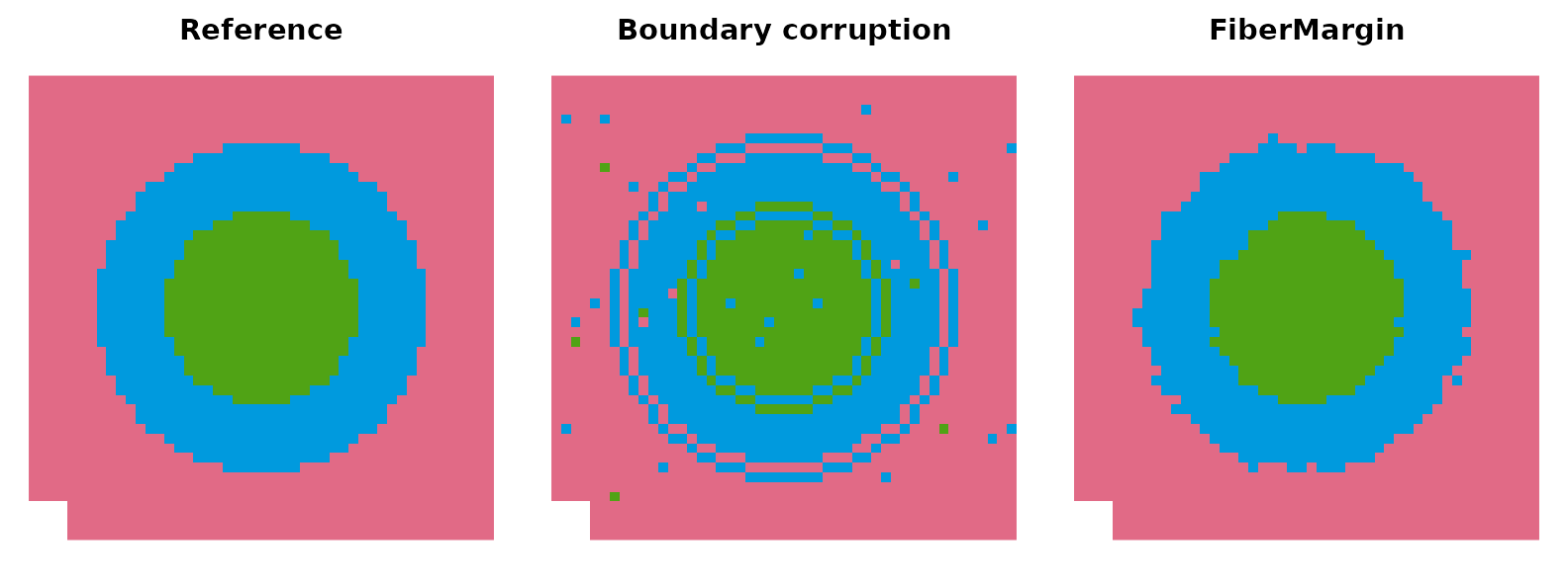

graphics::par(old_par)

A sample array can isolate sections inside one mask:

mask_samples <- matrix(
  ifelse(col(reference_mask) <= mask_size / 2, "left", "right"),
  nrow = mask_size, ncol = mask_size
)
cleaned_by_section <- clean_categorical_mask(
  initial_mask, samples = mask_samples, workers = 2L
)

The same API accepts a three-dimensional voxel array:

voxel_reference <- array("A", dim = c(20, 20, 8))
voxel_reference[, 8:14, ] <- "B"
voxel_reference[, 15:20, ] <- "C"
voxel_initial <- corrupt_categorical_mask(
  voxel_reference, mechanism = "boundary", rate = 0.10, seed = 9L
)
voxel_cleaned <- clean_categorical_mask(voxel_initial, workers = 2L)

`evaluate_mask_cleaning()`

Mask evaluation reports global recovery, ARI, class recall, correction and damage, mean and worst IoU, Dice, boundary IoU, and rare-class IoU.

mask_metrics <- evaluate_mask_cleaning(
  reference = reference_mask,
  initial = initial_mask,
  cleaned = cleaned_mask,
  method = "FiberMargin"
)

mask_metrics[, c(
  "method", "initial_accuracy", "accuracy", "ari",
  "mean_iou", "mean_boundary_iou", "rare_class_iou",
  "correction_recall", "damage_rate"
)]
#>        method initial_accuracy  accuracy       ari  mean_iou mean_boundary_iou
#> 1 FiberMargin        0.8500874 0.9759615 0.9300955 0.9453768         0.5329883
#>   rare_class_iou correction_recall  damage_rate
#> 1      0.9526814         0.8425656 0.0005141388

Accuracy obeys the exact repair-damage decomposition

with(
  mask_metrics,
  c(
    reported = accuracy,
    decomposed = initial_accuracy * (1 - damage_rate) +
      (1 - initial_accuracy) * correction_recall,
    numerical_error = repair_identity_error
  )
)
#>        reported      decomposed numerical_error 
#>    9.759615e-01    9.759615e-01   -1.110223e-16

Build and evaluate benchmark objects

`spatial_benchmark()`

Use spatial_benchmark() to validate custom coordinates and align all optional evaluation strata. Reference labels are stored for evaluation and are not passed to the repair function.

custom_benchmark <- spatial_benchmark(
  xy = gradient$xy,
  labels = gradient$labels,
  truth = gradient$truth,
  samples = gradient$samples,
  boundary = gradient$boundary,
  regions = gradient$area,
  sparse = gradient$sparse,
  name = "two_gradient_tissues",
  metadata = list(seed = 12L, purpose = "vignette")
)

class(custom_benchmark)
#> [1] "spatial_refinement_benchmark" "list"
names(custom_benchmark)
#> [1] "xy"       "labels"   "truth"    "samples"  "boundary" "regions"  "sparse"  
#> [8] "name"     "metadata"

boundary and sparse are optional logical vectors. If sparse is omitted but regions is supplied, evaluation uses the least frequent region as the sparse stratum and the most frequent region as the dense stratum.

`evaluate_spatial_refinement()`

This lower-level evaluator accepts aligned vectors and optional evaluation masks.

manual_metrics <- evaluate_spatial_refinement(
  truth = custom_benchmark$truth,
  initial = custom_benchmark$labels,
  refined = refined_gradient,
  boundary = custom_benchmark$boundary,
  regions = custom_benchmark$regions,
  sparse = custom_benchmark$sparse,
  elapsed = 0,
  method = "FiberMargin"
)

manual_metrics[, c(
  "accuracy", "accuracy_gain", "ari", "macro_recall", "worst_recall",
  "boundary_accuracy", "sparse_region_accuracy",
  "correction_recall", "damage_rate", "changed_precision"
)]
#>   accuracy accuracy_gain       ari macro_recall worst_recall boundary_accuracy
#> 1     0.98          0.08 0.9327002    0.9638053    0.9398496         0.9208333
#>   sparse_region_accuracy correction_recall damage_rate changed_precision
#> 1              0.9398496               0.9  0.01111111               0.9

Important measures are:

accuracy and ari: global recovery.
correction_recall: fraction of initially wrong labels repaired.
damage_rate: fraction of initially correct labels made wrong.
changed_precision: fraction of edited locations correct after repair.
macro_recall and worst_recall: class-balance diagnostics.
boundary_accuracy and sparse_region_accuracy: difficult-stratum outcomes.

`benchmark_spatial_refiners()`

A method is any function that accepts xy and labels; it may also accept samples or .... Every method receives identical input. The function accepts one benchmark or a named list of benchmarks.

jagged_small <- simulate_spatial_domains(
  n = 600L,
  pattern = "jagged_stripes",
  k = 4L,
  noise = 0.18,
  noise_type = "boundary",
  seed = 31L
)

comparison <- benchmark_spatial_refiners(
  data = list(
    gradient = custom_benchmark,
    jagged = jagged_small
  ),
  methods = list(
    FiberMargin = function(xy, labels, samples = NULL) {
      refine_spatial_labels(xy, labels, samples, workers = 1L)
    },
    IdentityExample = function(xy, labels, ...) labels
  ),
  include_initial = TRUE,
  seed = 5L,
  on_error = "stop"
)

comparison[, c(
  "dataset", "method", "accuracy", "ari",
  "correction_recall", "damage_rate", "seconds"
)]
#>    dataset          method  accuracy       ari correction_recall damage_rate
#> 1 gradient         Initial 0.9000000 0.6873537          0.000000  0.00000000
#> 2 gradient     FiberMargin 0.9800000 0.9327002          0.900000  0.01111111
#> 3 gradient IdentityExample 0.9000000 0.6873537          0.000000  0.00000000
#> 4   jagged         Initial 0.8200000 0.5837005          0.000000  0.00000000
#> 5   jagged     FiberMargin 0.8183333 0.5954988          0.537037  0.11991870
#> 6   jagged IdentityExample 0.8200000 0.5837005          0.000000  0.00000000
#>   seconds
#> 1   0.000
#> 2   0.005
#> 3   0.000
#> 4   0.000
#> 5   0.007
#> 6   0.000

Use on_error = "record" in long benchmark batches to retain a row containing the error message instead of stopping the entire run.

Simulation functions

Every simulator returns a spatial_refinement_benchmark-compatible list with xy, noisy labels, reference truth, and samples. Most also include boundary, sparse, region identifiers, and scenario metadata.

`simulate_spatial_clusters()`

This is the simplest geometry: separated Gaussian-like clusters in two or three dimensions. It is useful for smoke tests and binary-specialization examples.

cluster_sim <- simulate_spatial_clusters(
  n = 600L,
  dimensions = 3L,
  k = 4L,
  samples = 2L,
  noise = 0.10,
  seed = 2L
)
c(dimensions = ncol(cluster_sim$xy), classes = nlevels(cluster_sim$truth))
#> dimensions    classes 
#>          3          4
table(cluster_sim$samples)
#> 
#>   1   2 
#> 300 300

`simulate_spatial_domains()`

This simulator covers structured tissue geometries, corruption types, feature widths, density profiles, and multiple specimens.

Available patterns are jagged_stripes, wavy_layers, rings, spiral, branching, lobes, islands, disconnected, thin_layers, intermixed, and layers3d. Only layers3d uses three dimensions. Corruption can be random, boundary, patch, or region. Density can be uniform, moderate, strong, extreme, hotspot, or a positive weight per class.

domain_sim <- simulate_spatial_domains(
  n = 800L,
  pattern = "thin_layers",
  k = 5L,
  noise = 0.20,
  dimensions = 2L,
  samples = 2L,
  noise_type = "boundary",
  feature_scale = 0.8,
  density_profile = "strong",
  seed = 3L
)
table(domain_sim$truth)
#> 
#> cluster1 cluster2 cluster3 cluster4 cluster5 
#>      753        6       16       18        7

`simulate_complex_spatial_domains()`

This held-out geometry family stresses junctions, narrow channels, non-convex boundaries, and severe class-density imbalance. Shapes are voronoi_mosaic, radial_sectors, checkerboard_junctions, tubular_network, braided_channels, and shells_3d.

complex_sim <- simulate_complex_spatial_domains(
  n = 700L,
  shape = "tubular_network",
  density_profile = "extreme",
  noise_type = "patch",
  noise = 0.20,
  samples = 1L,
  k = 5L,
  seed = 4L
)
c(dimensions = ncol(complex_sim$xy), observations = nrow(complex_sim$xy))
#>   dimensions observations 
#>            2          700

`simulate_gradient_regions()`

This function generated the quick-start object. It supports 2D or 3D coordinates, multiple tissues, curved boundaries, and custom area-density weights.

gradient_3d <- simulate_gradient_regions(
  n = 700L,
  minority = 0.05,
  dimensions = 3L,
  samples = 2L,
  seed = 5L,
  curvature = 0.06,
  density_profile = c(1, 2, 0.5, 3)
)
table(gradient_3d$area, gradient_3d$truth)
#>        
#>           A   B   C
#>   area1 104   0   0
#>   area2   0 223   0
#>   area3   0  55   0
#>   area4   0   0 318

`simulate_volumetric_domains()`

This is the dedicated 3D stress-test generator. Available shapes are concentric_shells, warped_ellipsoids, toroidal_compartments, folded_layers, thin_folded_sheets, branching_tubes, disconnected_volumes, and helical_channels.

Acquisition can be uniform, class_imbalanced, or irregular_z; corruption can be random, boundary, patch, or region.

volume_sim <- simulate_volumetric_domains(
  n = 700L,
  shape = "folded_layers",
  acquisition = "class_imbalanced",
  noise_type = "boundary",
  noise = 0.20,
  k = 5L,
  samples = 2L,
  seed = 6L
)

c(
  dimensions = ncol(volume_sim$xy),
  observations = nrow(volume_sim$xy),
  samples = nlevels(volume_sim$samples)
)
#>   dimensions observations      samples 
#>            3          700            2
volume_sim$region_counts
#> region
#> region1 region2 region3 region4 region5 
#>      46     391      35      69     159

old_par <- graphics::par(no.readonly = TRUE)
graphics::par(mfrow = c(2, 2), mar = c(3, 3, 2, 1))
plot_field(cluster_sim$xy, cluster_sim$truth, "Spatial clusters", cex = 0.45)
plot_field(domain_sim$xy, domain_sim$truth, "Thin layers", cex = 0.45)
plot_field(complex_sim$xy, complex_sim$truth, "Tubular network", cex = 0.45)
plot_field(volume_sim$xy, volume_sim$truth, "3D folded layers: x-y", cex = 0.45)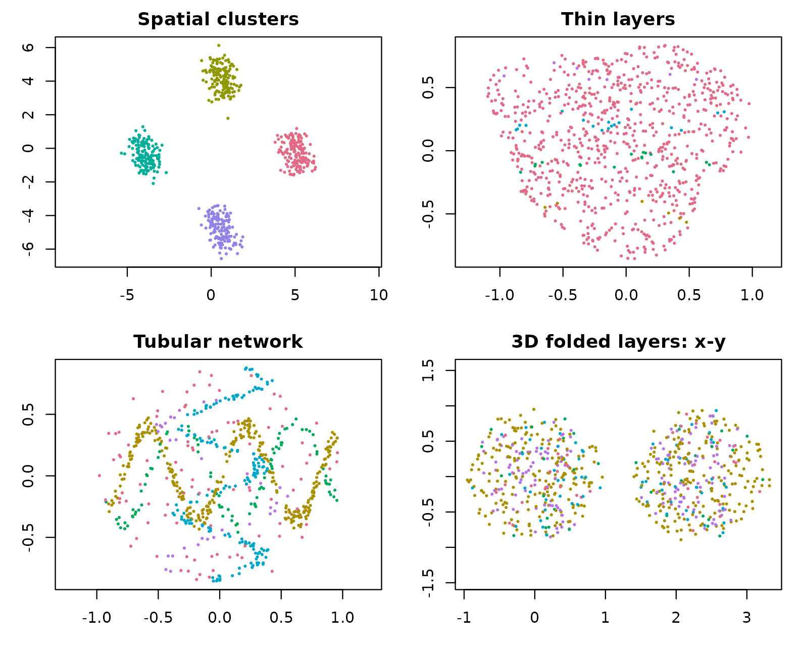

graphics::par(old_par)

Bundled real benchmarks

`available_spatial_benchmarks()`

Always inspect availability and licensing before requesting a real dataset:

benchmark_status <- available_spatial_benchmarks()
benchmark_status[c(
  "dataset", "included", "observations", "classes", "scenarios"
)]
#>   dataset included observations classes scenarios
#> 1   dlpfc     TRUE        47329       7        45
#> 2 merfish    FALSE        28317       8        45
#> 3     crc     TRUE       194541      19        60

DLPFC and CRC are bundled as coordinate-and-label derivatives. Expression matrices and tissue images are excluded. MERFISH is listed for provenance but cannot be redistributed with the package because the derived annotation does not have an explicit redistribution license. The complete object also records the license, source, and note fields for every dataset.

`load_spatial_benchmark()`

Load a bundled scenario by integer position:

dlpfc_case <- load_spatial_benchmark("dlpfc", scenario = 1L)
c(
  observations = nrow(dlpfc_case$xy),
  classes = nlevels(dlpfc_case$truth),
  specimens = nlevels(dlpfc_case$samples),
  input_accuracy = mean(dlpfc_case$labels == dlpfc_case$truth)
)
#>   observations        classes      specimens input_accuracy 
#>   4.732900e+04   7.000000e+00   1.200000e+01   9.499884e-01
dlpfc_case$scenario
#>   noise      mechanism replicate scenario_index    seed
#> 1  0.05 interface_band         1              1 7315001
#>                  scenario_id changed_observations actual_error
#> 1 DLPFC_interface_band_05_r1                 2367   0.05001162
#>   boundary_enrichment
#> 1            3.211304

Scenario identifiers are also accepted:

crc_case <- load_spatial_benchmark(
  "crc", scenario = "CRC_random_25_r1", seed = 1040001L
)
crc_refined <- refine_spatial_labels(
  crc_case$xy, crc_case$labels,
  samples = crc_case$samples,
  workers = 4L
)
evaluate_spatial_refinement(
  crc_case$truth, crc_case$labels, crc_refined,
  boundary = crc_case$boundary,
  sparse = crc_case$sparse,
  method = "FiberMargin"
)

The legacy dataset name "colorectal" is accepted as an alias for "crc". Calling load_spatial_benchmark("merfish") intentionally reports why that dataset is not bundled.

End-to-end analysis template

The following pattern can be adapted to a real coordinate-indexed annotation:

# One row per spatial location.
xy <- as.matrix(my_data[, c("x", "y")])
labels <- factor(my_data$annotation)
samples <- factor(my_data$section_id)

# Repair does not receive the reference labels.
refined <- refine_spatial_labels(
  xy = xy,
  labels = labels,
  samples = samples,
  workers = 4L
)

# Inspect edits before replacing an annotation column.
audit <- data.frame(
  observed = labels,
  candidate = attr(refined, "candidate"),
  refined = refined,
  changed = attr(refined, "changed"),
  margin_score = attr(refined, "margin_score"),
  required = attr(refined, "required"),
  repair_margin = attr(refined, "repair_margin"),
  isolation = attr(refined, "isolation")
)

my_data$fibermargin_annotation <- refined

When an independent reference is available, evaluate correction and damage together:

evaluate_spatial_refinement(
  truth = reference_labels,
  initial = labels,
  refined = refined,
  boundary = boundary_locations,
  sparse = rare_or_sparse_locations,
  method = "FiberMargin"
)

Reporting checklist

For reproducible analyses, report:

Coordinate dimension and number of locations.
Number of classes and independent specimens.
Whether the binary specialization or multiclass enclosure mechanism was used.
The workers budget and package version.
Accuracy and ARI when a reference exists.
Correction recall and damage rate together.
Boundary, sparse-region, macro-recall, and worst-recall diagnostics when relevant.
The unchanged input, repaired labels, and pointwise audit attributes.

Function-level argument and return-value details remain available through help(package = "fibermargin") and ?function_name.

FiberMargin authors

Purpose and input contract

Quick start

Refine irregular coordinates

refine_spatial_labels()

Binary specialization

Effective 2D and genuine 3D coordinates

Multiple specimens

Deterministic CPU use

Clean categorical masks

corrupt_categorical_mask()

clean_categorical_mask()

evaluate_mask_cleaning()

Build and evaluate benchmark objects

spatial_benchmark()

evaluate_spatial_refinement()

benchmark_spatial_refiners()